Cell Annotation
Statistical analysisCell annotation is the process of assigning labels to the cell clusters, by linking their transcriptionnal signatures to the cell type, state, function, location or lineage they reflect. The main challenges of cell annotation are first to extract a relevant list of marker genes that are specifically characterising the expression profils, and then associate those markers to biological meaning based on empirical knowledge. As this task can be quite laborious, label transfer methods leveraging on already annotated datasets can be use to facilitate the process.
Module specifications
| Input data | Computationnal environnement | Output data |
|---|---|---|
|
annotated data matrices |
scRNA-seq_data_analysis R |
annotated data matrices |
Code
This module is based on the following documentation :
Seurat v4 R package
Hao Y, Hao S, Andersen-Nissen E, et al. Integrated analysis of multimodal single-cell data. Cell. 2021;184(13):3573-3587.e29. doi:10.1016/j.cell.2021.04.048
* https://satijalab.org/seurat/articles/get_started.html
* https://htmlpreview.github.io/?https://github.com/satijalab/seurat.wrappers/blob/master/docs/harmony.html
Guidelines for scRNA-seq analysis
Luecken MD, Theis FJ. Current best practices in single-cell RNA-seq analysis: a tutorial. Mol Syst Biol. 2019;15(6):e8746. Published 2019 Jun 19. doi:10.15252/msb.20188746
* https://pubmed.ncbi.nlm.nih.gov/31217225/
This module require to load the following environment of R packages :
source("/home/truchi/Starter_pack.R")
Informations about the demo dataset :
The demo dataset is a collection of 18 public 10X Genomics Chromium samples (GSE151374) of control (n=6) or bleomycin-treated mice lungs (n=12), collected after 7 or 14 days following treatment. Half of bleomycin-treated mice were also treated with Nintedanib, an anti-fibrotic drug (see associated publication).
This dataset has already been processed (see the "Integration of multiple scRNA-seq samples" module).
Notes
Annotation often requires extensive and time-consuming work, even when data analysts or their collaborators are experts of the studied system. Indeed, trying to recognize single-cell transcriptomics signatures using genes identified as markers through their protein expression, like surface markers, may not be successful due to the limited correlation between protein and gene expression measurements. Moreover, while most identified markers are usually functionally-annotated coding genes, these annotations may not provide information on contextual cell identity or function. Finally, some signatures may reflect unwanted variability, induced by technical bias, and confuse the annotation.
1. Load a scRNA-seq dataset and compute top markers table
Here we load the seurat object saved after integration of 18 lung samples from PBS or bleomycin-treated mice.
aggr <- readRDS("/data/analysis/data_truchi/GSE151374.rds")
The biological relevance of identified clusters is evaluated by manually inspecting the expression pattern of known genes or by measuring differences in gene expression between cells in each cluster and the rest of the dataset.
The table of most differentially expressed genes per cluster can be obtained with the FindAllMarkers seurat function.
This function ranks in ascending order the mean normalized and log-transformed expression values of a gene in all cells of both groups (a particular cluster vs all other clusters).
The sums of the ranks obtained for each group are then calculated, along with the probability of observing identical or more extreme values, on the assumption that there is no difference between the two groups being compared (Wilcoxon rank test).
As these pvalues are calculated for several thousand genes, a Bonferroni adjustment is applied to prevent the increase in type 1 error inherent to multiple testing.
# Differential expression analysis between a cluster and the rest for all clusters
# logfc.threshold = 0.8 -> only keep genes this a |log2FC| > 0.8
# min.pct = 0.5 -> only keep genes that are at list detected in 50% of cells of the cluster
# only.pos = T -> only keep over-expressed genes
markers <- FindAllMarkers(aggr,logfc.threshold = 0.8,min.pct = 0.5,only.pos = T)
markers
                 p_val avg_log2FC pct.1 pct.2     p_val_adj cluster     gene
Gpihbp1   0.000000e+00  3.6755411 0.890 0.088  0.000000e+00       0  Gpihbp1
Plvap     0.000000e+00  3.5183490 0.778 0.069  0.000000e+00       0    Plvap
Clec14a   0.000000e+00  3.4793951 0.853 0.084  0.000000e+00       0  Clec14a
Tspan7    0.000000e+00  3.2194509 0.904 0.114  0.000000e+00       0   Tspan7
Tm4sf1    0.000000e+00  3.1688342 0.756 0.080  0.000000e+00       0   Tm4sf1

# Save it in an excel file
write.xlsx(markers,"top_markers.xlsx")
The avg_log2FC is the log2 of the ratio between the mean expression in the cluster and the mean expression in all other clusters.
The column pct.1 and pct.2 indicated the percentage of cells with at list 1 count for the gene in the cluster and in all other cells respectively.
As we are looking for markers of very distinct populations and comparing several thousands of cells, the computed pvalues are often very low (R is even often displaying "0.000000e+00" as it can't display too small numbers).
# Show the most differentially expressed gene per cluster in a dotplot, which display both the expression level and the % of cells expressing the gene
best.markers <- markers %>% dplyr::group_by(cluster) %>% dplyr::slice_max(avg_log2FC,n=1) %>% pull(gene) %>% unique()
DotPlot(aggr, features = best.markers,group.by = "seurat_clusters") + geom_point(aes(size=pct.exp), shape = 21, colour="black", stroke=0.5) +
  scale_colour_viridis(option="magma") + guides(size=guide_legend(override.aes=list(shape=21, colour="black", fill="white")))+ylab("")+xlab("")+ RotatedAxis()+FontSize(x.text = 10,y.text = 10)
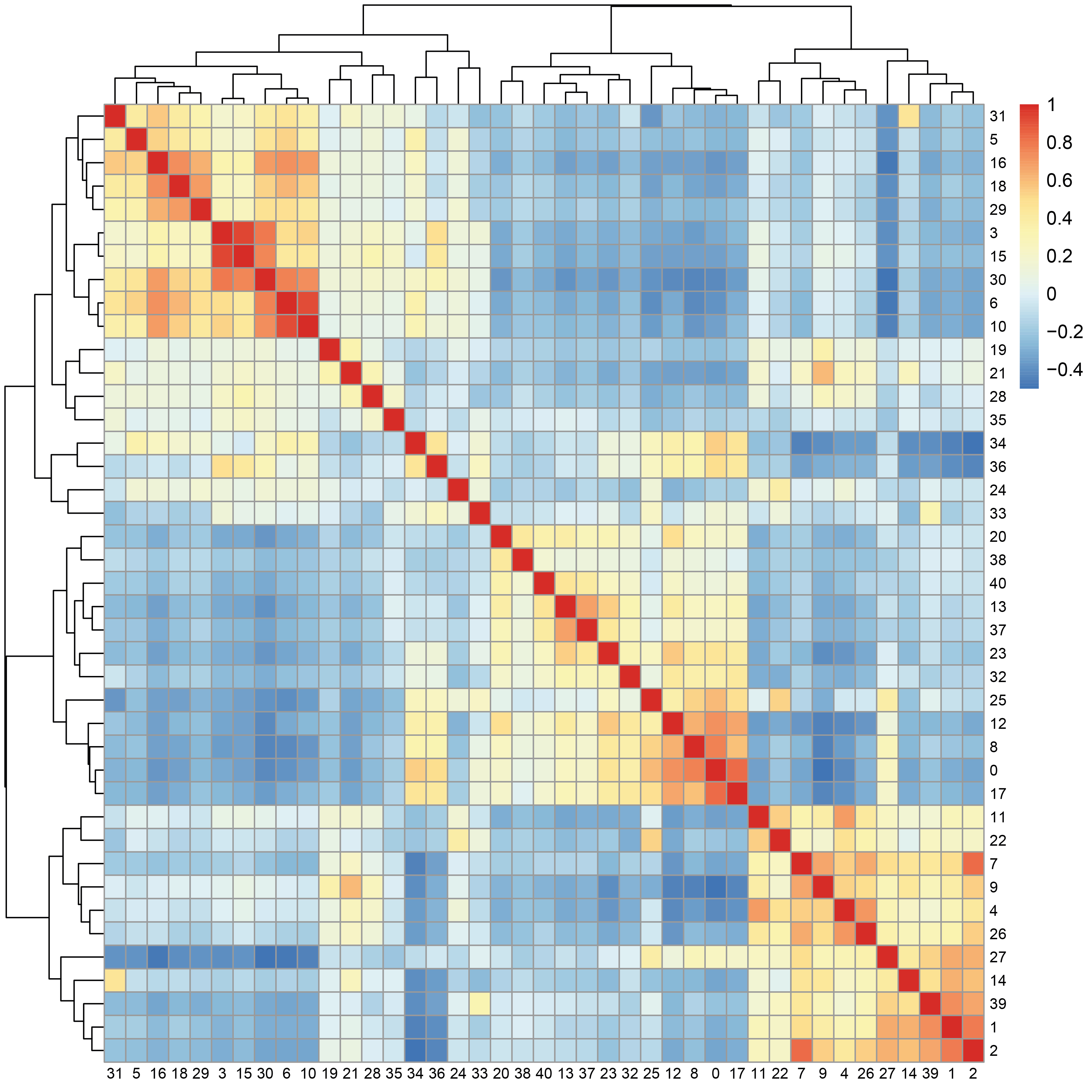
The matrix of correlation between average expression profiles of top markers in each cluster indicates which clusters are sharing similar signatures.
average <- AverageExpression(aggr,group.by = "seurat_clusters",return.seurat = T,features = unique(markers$gene))
data <- GetAssayData(average,slot = "scale.data")
corr.data <- cor(data)
2. Use an already annotated reference to automatically transfer labels
Ideally, a biologically relevant cluster has a signature of multiple markers that are strongly and specifically expressed, with explicit functions that help to identify the corresponding cell population.
However, this ideal situation is rarely found for all clusters.
Indeed, some are characterized by overexpressed but non-specific genes, or by highly specific but undetermined genes.
Moreover, some clusters may have a distinct but artefactual signature, resulting from technical biases and/or over-clustering.
To overcome these problems, the idea is to use pre-existing, publicly available annotations.
Datasets deposited on "Gene Expression Omnibus" or other public repositories should contain both the counts annotations, either associated in analysis object (such as sce, anndata or seurat) or separated in distinct tables.
However, the reference and the query datasets should be similarly processed and under the same format.
In the following example, we use the transfer annotation method implemented in seurat, to transfer the annotation of a published dataset of the same bleomycin mice model into the query un-annotated dataset.
The general idea is to find anchor points between reference and query, i.e. pairs of mutual nearest neighbors cells in the two datasets, which are weighted according to the number of mutual nearest neighbors pairs in their vicinity.
The weighted anchors are then used to predict the potential annotation of each query cell based on its anchors neighborhood..
# Load the reference dataset as a seurat object containing the annotated cells
ref <- readRDS("/data/analysis/data_hermet/bleo_dissociated_ref.rds")

# The dimensions of the reference dataset must have been reduced by pca before running the integration
anchors <- FindTransferAnchors(reference = ref, query = aggr,dims = 1:80, reference.reduction = "pca")
predictions <- TransferData(anchorset = anchors, refdata = ref$celltype,dims = 1:80)
# This function add, in the metadata of the query dataset, a column corresponding to the predicted score for each reference label, as well as a "predicted.id" column corresponding to the label with the highest predicted score
aggr <- AddMetaData(aggr, metadata = predictions)

# Plot simultaneously the seurat clusters and the predicted
colors.Bleo<- c("AM1"="#7FCDBB","AM2"="#41B6C4","AM3"="#1D91C0","IM"="#225EA8",
                "cDC1"="#e670b4","cDC2"="#9c119c","Mature DC"="#960c5a","pDC"="#de439a","cMonocytes"="#66119c","ncMonocytes"="#282b5c","Neutrophils"="#4300de","Mast cells"="#9315ed","Platelets"="#de1212","RBC"="#de1212",
                "CD4 T cells"="#D9F0A3","Reg T cells"="#ADDD8E","T helper cells"="#78C679","Gamma delta T cells"="#41AB5D","ILC2"="#739154","CD8 T cells"="#006837" ,"NKT1"="#01736b","NKT2"="#01738c","NK cells"="#46c798","B cells"="#ebd513","Plasmocytes"="#ccbf47",
                "gCap"="#911414","aCap"="#752740","Venous EC"="#f2ae5a","Arterial EC"="#e37e12","Lymphatic EC"="#7d3f15","Fibroblasts"="#d3d5db","Myofibroblasts"="#656566","Pericytes"="#806c6c",
                "Mesothelial cells"="#120c04","AT1"="#8184b8","AT2"="#3e447a","Ciliated cells"="#1486f7","Club cells"="#c5edea","Goblet cells"="#60807d","Krt8 ADI"="#fa8750",
                "Proliferating cells"="#e6f7f7")
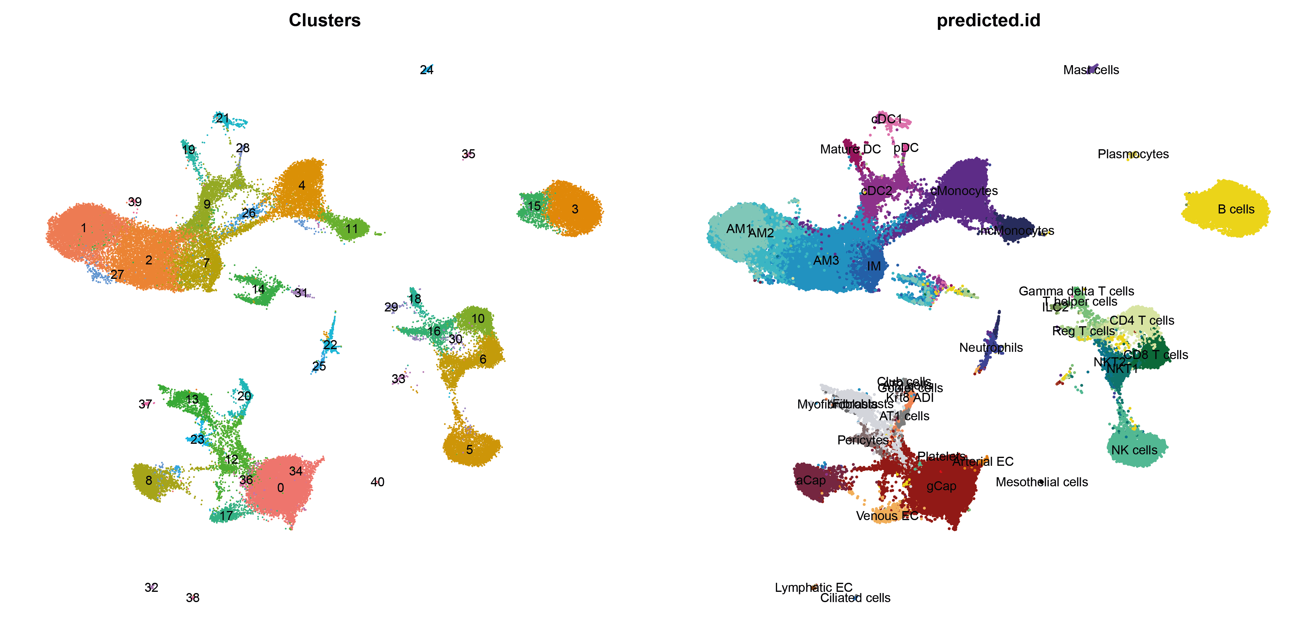
p1 <- DimPlot(object = aggr, group.by = "seurat_clusters",reduction = "umap", label=TRUE)+ ggtitle("Clusters")+NoAxes()+NoLegend()
p2 <-DimPlot(object = aggr,group.by = "predicted.id",  reduction = 'umap', label = T,cols = colors.Bleo, pt.size = 0.5)+NoAxes()+NoLegend()
plot_grid(p1,p2,ncol = 2)
3. Leverage on automatic label transfer to annotate the clusters
3.1 Assign relevant labels
The automatic label transfer should not be used as a definitive annotation, as :
- some query dataset clusters may represent a biological signature absent in the reference
- some predicted labels may not be relevant in the query dataset
For instance, based on the plots above, it appears that clusters 14 and 31 have been assigned to a mix of myeloid and lymphoid cells populations, meanwhile those clusters bring a cell cycle signature which wasn't present in the reference.
It is therefore preferable to annotate them differently from other cells of the same lineage, as they reflect a different biological state.
Reversely, the reference dataset captured a signature of alveolar macrophages (AM2), which corresponded to an intermediate phenotype between tissue-resident alveolar macrophages (TR-AM) and monocytes-derived alveolar macrophages (MD-AM), therefore respectively labeled as "AM1" and "AM3" in the reference.
However, this intermediate state seems not detected as a singular cluster in the query dataset, and appears mixed with AM1.
It is therefore preferable not to keep the same nomenclature as in the reference, but rather to use one more in line with the 2-pole distribution of alveolar macrophages in the query dataset.
More generally, the idea is to ajust the annotation depending on the focus of the analysis.
For instance, the analysis modules based on this annotation step will not focus on lymphocytes or epithelial cells.
It is thefore relevant to gather sub-populations (ex : "Cd4 T cells", "Cd8 T cells", "T helper cells") under a coarser label (ex : "T cells") to simplify the process.
These coarser labels can also be use to gather clusters with unclear signatures that must be inspected more deeply.
aggr$clusters <- Idents(aggr)
aggr$clusters <- factor(aggr$clusters, levels =c("0","1","2","3","4","5","6","7","8","9","10","11","12","13","14","15","16","17","18","19","20","21","22","23","24","25","26","27","28","29","30","31","32"))
Idents(aggr) <- "clusters"

new.cluster.ids <- c("gCap","TR-AM","MD-AM","B cells","cMonocytes","NK cells","T cells","IM","aCap","cDC2","T cells","ncMonocytes","unclear",
                     "Fibroblasts","Prolif. Immune cells","B cells","T cells","Venous EC","T cells","Mature DC","Epithelial cells","cDC1","Neutrophils",
                     "Pericytes","Mast cells","Neutrophils","IFN-Monocytes","unclear","pDC","T cells","unclear","Prolif. Immune cells","Lymphatic EC",
                     "RBC","unclear","Plasma cells","unclear","Fibroblasts","Epithelial cells","RBC","Mesothelial cells")
names(x = new.cluster.ids) <- levels(x = aggr)
aggr <- RenameIdents(object = aggr, new.cluster.ids)

DimPlot(object = aggr,  reduction = 'umap', label = T,cols = colors.Bleo, pt.size = 0.5)
aggr$celltype <- Idents(aggr)
3.2 Subcluster to refine the annotation
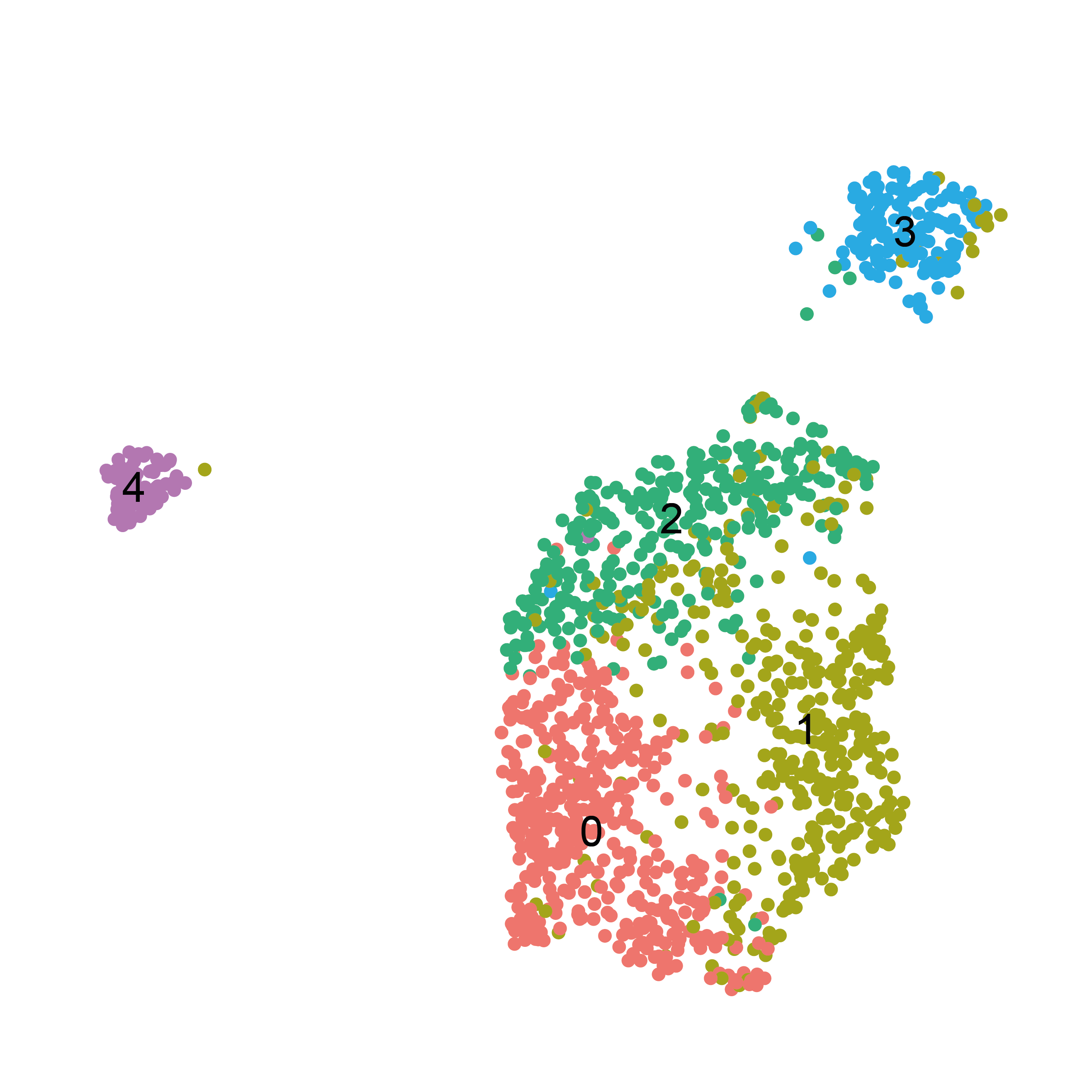
The idea is to perform a sub-clustering of a targeted subset of cells in order to capture cell communities whose signatures may have been hidden in the global clustering by the use of too small a resolution.
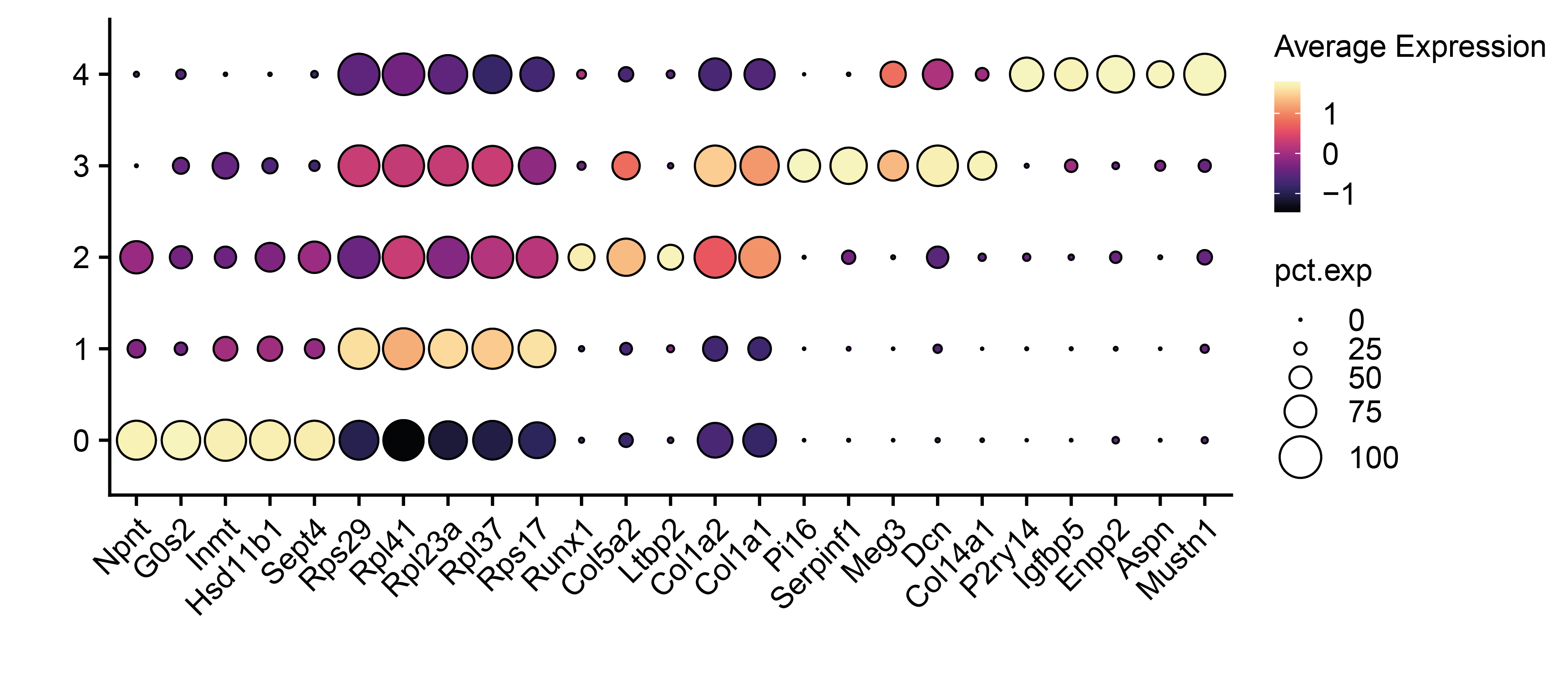
For instance, the subclustering of fibroblasts reveals a more complex phenotypes repartition, which has been described to reflect their location in the tissue.
# Extract the recently-annotated Fibroblasts subset
sub <- subset(aggr,idents=c("Fibroblasts"))
# Rerun the clustering based on the already computed space of 100 harmony's dimensions
sub <- FindNeighbors(sub, reduction = "harmony", dims = 1:100,k.param = 10)
sub <- FindClusters(sub, resolution = 0.2)
sub <- RunUMAP(sub, reduction = "harmony", dims = 1:100)
DimPlot(sub, group.by = c("seurat_clusters"),label = T)+NoAxes()+NoLegend()
# To support the annotation of subclusters, find their markers
markers <- FindAllMarkers(sub,logfc.threshold = 0.5,min.pct = 0.5,only.pos = T)

# Show the top 5 differentially expressed markers for each subcluster
best.markers <- markers %>% dplyr::group_by(cluster) %>% dplyr::slice_min(p_val_adj,n=5) %>% pull(gene) %>% unique()
DotPlot(sub, features = best.markers,group.by = "seurat_clusters") + geom_point(aes(size=pct.exp), shape = 21, colour="black", stroke=0.5) +theme(legend.title = element_text(size = 10),legend.text = element_text(size = 10),legend.key.size = unit(0.3, 'cm'))+
  scale_colour_viridis(option="magma") + guides(size=guide_legend(override.aes=list(shape=21, colour="black", fill="white")))+ylab("")+xlab("")+ RotatedAxis()+FontSize(x.text = 10,y.text = 10)
# Assign their new annotation
select.cells <- names(Idents(sub)[which(Idents(sub) %in% c(0,1,2))])
aggr <- SetIdent(object = aggr, cells = select.cells, value = "Alveolar.F")
select.cells <- names(Idents(sub)[which(Idents(sub) %in% c(3))])
aggr <- SetIdent(object = aggr, cells = select.cells, value = "Adventitial.F")
select.cells <- names(Idents(sub)[which(Idents(sub) %in% c(4))])
aggr <- SetIdent(object = aggr, cells = select.cells, value = "Peribronchial.F")
aggr$celltype <- Idents(aggr)
3.3 Remove unwanted cells and finalize the annotation
After clustering and annotation process, some labels could have been associated to expression profiles reflecting noise and technical bias, that are therefore unwanted for downstream analysis.
Those profiles may correspond to potential doublets, unviable cells, dissociation-induced stressed signatures, cells that should not have been captured etc ...
Here, they have been gathered under the "unclear" label. Red blood cells, which are not supposed to be sequenced, will be discared too.
# Remove noisy signatures and Red Blood Cells
aggr <- subset(aggr,subset=celltype %ni% c("RBC","unclear"))

# Define the final celltype palette and ordering for plots
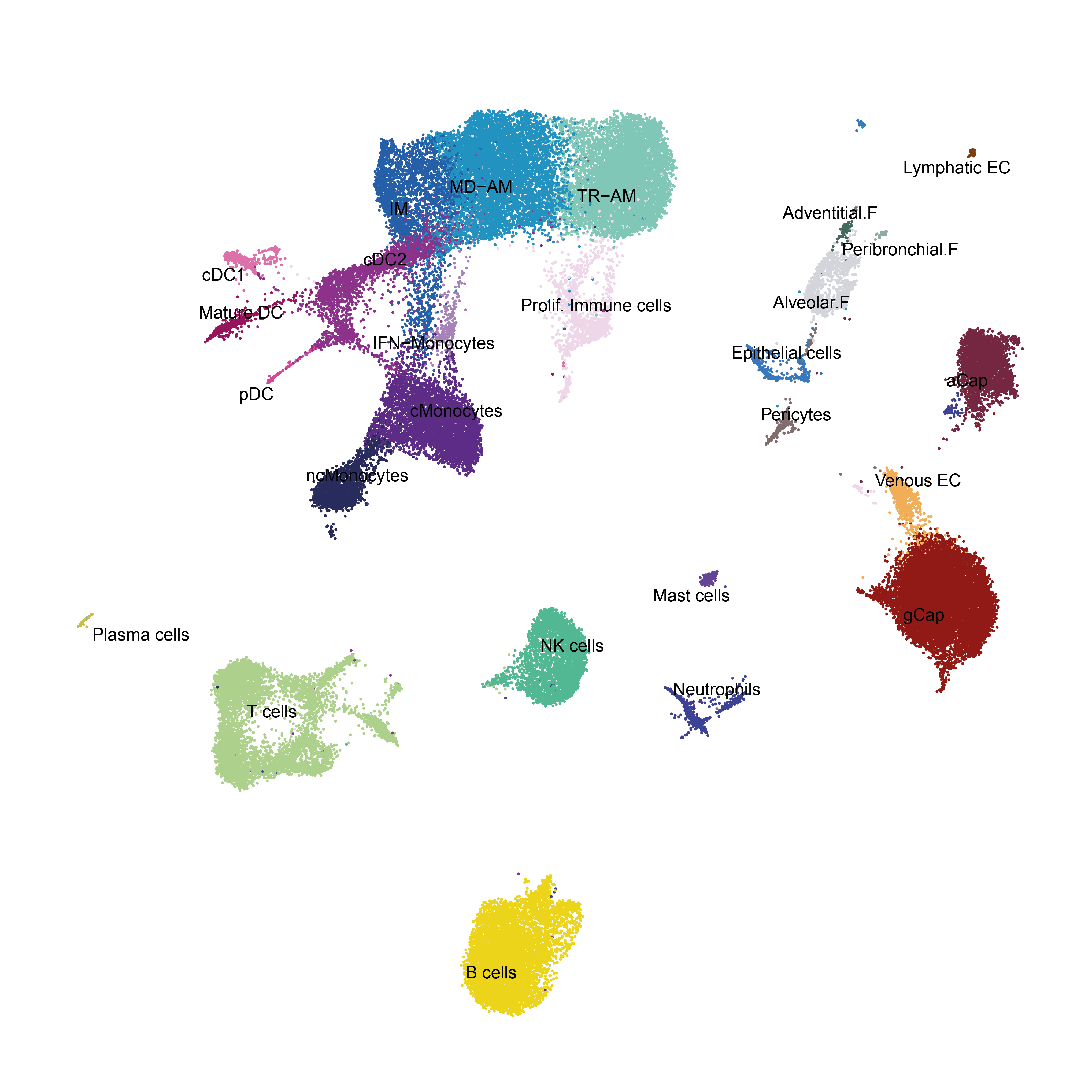
colors.Bleo<- c("TR-AM"="#7FCDBB","MD-AM"="#1D91C0","IM"="#225EA8","IFN-Monocytes" = "#aa83c7","cMonocytes"="#66119c","ncMonocytes"="#282b5c","Prolif. Immune cells"="#f0d8ee",
                "Mature DC"="#960c5a","cDC1"="#e670b4","cDC2"="#9c119c","pDC"="#de439a","Neutrophils"="#4300de","Mast cells"="#9315ed",
                "T cells"="#ADDD8E","NK cells"="#46c798","B cells"="#ebd513","Plasma cells"="#ccbf47",
                "Prolif. EC"="#f2d0d0","gCap"="#911414","aCap"="#752740","Venous EC"="#f2ae5a","Lymphatic EC"="#7d3f15",
                "Alveolar.F"="#d3d5db","Adventitial.F"="#436b5d","Peribronchial.F"="#90ada3","Pericytes"="#806c6c","Epithelial cells"="#1486f7")
celltype_order <- names(colors.Bleo)
aggr$celltype <- factor(as.character(aggr$celltype),levels = celltype_order)

# Rerun the UMAP with the final selection of cells
aggr <- RunUMAP(aggr, reduction = 'harmony', dims = 1:100)
DimPlot(aggr,group.by = "celltype",cols = colors.Bleo,label = T,repel = T,label.size = 3)+NoAxes()+NoLegend()

# Choose the "celltype" annotation as default identity
Idents(aggr) <- "celltype"

# Save the final analysis object
saveRDS(aggr,file = "/data/analysis/data_truchi/GSE151374.rds")
