Index

Cytometry-differential_abundance_analysis

Cytometry Single-cell Statistical analysis

Differential analysis of cell population abundance is conducted to compare cell type proportions across experimental conditions, with statistical results visualized through boxplots. Tests for differential abundance of clusters are calculated using generalized linear mixed models implemented in the diffcyt R package.

Module specifications

Input data	Computational environnement	Output data
annotated data matrices	Cytometry_data_analysis R	annotated data matrices, differential analysis table

Code

This module is based on the following documentation :

CyTOF workflow, a suite of R packages to analyse cytometry data
Nowicka M, Krieg C, Crowell HL, Weber LM, Hartmann FJ, Guglietta S, Becher B, Levesque MP, Robinson MD. CyTOF workflow: differential discovery in high-throughput high-dimensional cytometry datasets. F1000Res. 2017 May 26;6:748. doi: 10.12688/f1000research.11622.3.
* https://www.bioconductor.org/packages/release/workflows/vignettes/cytofWorkflow/inst/doc/cytofWorkflow.html#data-import "CyTOF workflow"

diffcyt, a R package for differential discovery analyses in high-dimensional cytometry data
Weber LM, Nowicka M, Soneson C, Robinson MD. diffcyt: Differential discovery in high-dimensional cytometry via high-resolution clustering. Commun Biol. 2019;2:183. Published 2019 May 14. doi:10.1038/s42003-019-0415-5
* https://bioconductor.org/packages/release/bioc/vignettes/diffcyt/inst/doc/diffcyt_workflow.html

This module require to load the following environment of R packages :

source("/data/analysis/data_truchi/Cytometry/ODIN/cytometry_R_packages.R")

Informations about the demo dataset :

The demo dataset results from a standard flow cytometry experiment, containing 5 sham, 5 stimulated samples and 1 naïve sample.

Notes

This module expects as input a SingleCellExperiment object containing the (transformed) matrix of protein abundance associated to the refined cell annotation obtained after running the the high resolution clustering module.

The differential analysis of markers expression is not covered in the cytometry data analysis pipeline.
Indeed, the markers chosen for the demo dataset are all celltype's markers that are not expected to be differentially expressed between conditions.
Moreover, the diffcyt functions dedicated to the differential analysis are designed to run on sce object that only take into account the original 20 FlowSOM clusters.
However, if your dataset is suitable for this type of differential analysis on the 20 FlowSOM clusters, follow the instructions of the CytoF vignette

Load a SingleCellExperiment object and convert it to Seurat and SummarizedExperiment

The SingleCellExperiment class is a S4 R object dedicated for single-cell data handling, containing both the quantitative measures and the cells/features annotations.
It is the expected output of the high resolution clustering module. However, for representation purpose and to run the differential abundance analysis on each particular subpopulation, we will convert it to both Seurat and SummarizedExperiment objects, 2 others popular classes used for single-cell data analysis in R.

# Open the SingleCellExperiment object stored in .rds file
sce <- readRDS("cytometry_sce.rds")

Visualise the relative proportions of each subpopulation in each sample

#  Transform it into a seurat object
data <- sce@assays@data@listData[["exprs"]]
data <- as(data,"dgCMatrix")
metadata <- colData(sce) %>% as.data.frame()
rownames(metadata) <- metadata$barcode
colnames(data) <- metadata$barcode
seuratobj <- CreateSeuratObject(counts = data,meta.data = metadata,min.cells = 0,min.features = 0)

# Define the cluster color palette 
colors.NH <- c("Conv. Naive CD8"="#da3b5e","Inf. Naive CD8"="#e58289","Conv. Effector CD8"="#a34c4f","Inf. Memory CD8"="#d04336","NK cells"="#a4532b","NKT"= "#e06e34","g/d Treg"="#d99634","g/d T1"="#806a2b","g/d T17"="#bdb02e","Conv. Naive CD4 T cells"="#85b937","Naive Treg"="#81b66c","Conv. Effector Th1"="#3a8f36","Conv. Effector Th17"="#3a6e3a","Activated Effector T cells"="#4cc45b","Activated Effector Treg"="#54c79a","Activated Memory Treg"="#3d9472", "Memory B cells"="#42c0c7","Marginal Zone B cells"="#50a4d3","B1a cells"="#7395e4","Plasmablast"="#cdccfc","Plasma cells"="#6563d9", "MZMacro"="#092973","RPMacro"="#0289e3","MMMacro"="#b8e4f5","CD11B- Myeloid cells"="#8e68c7","CMonocytes"="#d196d6","IMonocytes"="#a43aac","NCMonocytes"="#d86edb","Neutrophils"="#9c659a","Mast cells"="#750067","Mature pDC"="#974b6d","CD11B+ cDC"="#de4c98","CD8+ cDC"="#b53d6c","unknow"="grey")

# Extract the proportions from the cells annotations table                           
metadata <- seuratobj@meta.data
metadata = as.data.frame.matrix(table(metadata$sample_id, metadata$celltype))
metadata = as.data.frame(metadata / rowSums(metadata))
metadata$sample_id = rownames(metadata)

metadata = gather(metadata, celltype, percentage, 'Conv. Naive CD8':'CD8+ cDC')

# Order the samples
metadata$sample_id =factor(metadata$sample_id, levels = c("A11-Naive","A1-NS1" ,"A2-NS2","A3-NS3","A4-NS4","A5-NS5","A6-S1","A7-S2","A8-S3","A9-S4","A10-S5"))

df <- seuratobj@meta.data[,c("sample_id","condition")] %>% unique()
metadata <- inner_join(metadata,df)

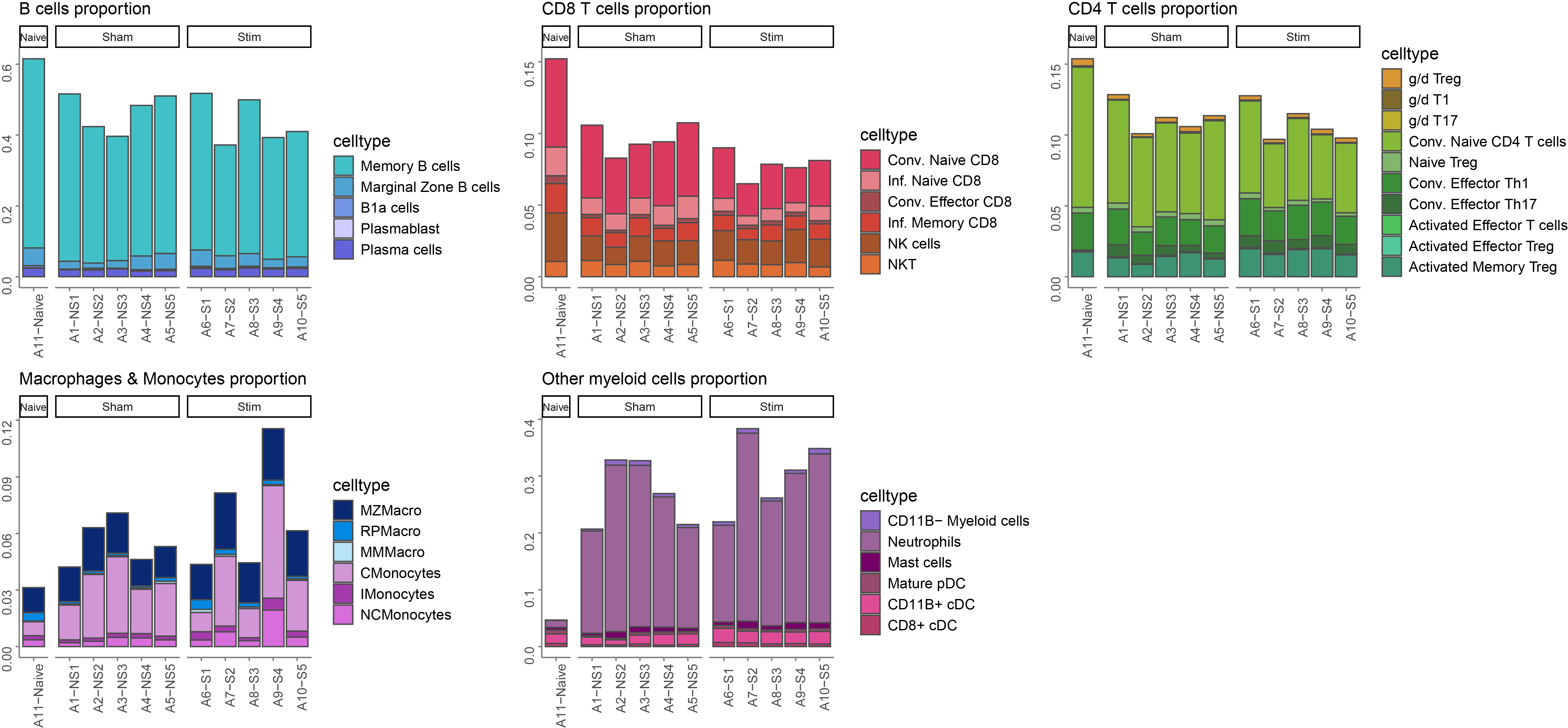
Groups of related celltypes are plotted separately for clarity.

# B cells group
Bcells <- metadata %>% dplyr::filter(celltype %in% c("Memory B cells","Marginal Zone B cells","B1a cells","Plasmablast","Plasma cells"))
p1 <- ggplot(Bcells, aes(x = sample_id, y = percentage, fill = celltype)) +
  geom_bar(stat = 'identity', color = "grey30") + facet_grid(~condition, scales = "free_x", space = "free_x") +
  ggtitle("B cells proportion")+
  scale_fill_manual(values = colors.NH) +
  theme_classic() +
  theme(axis.text.x = element_text(size = 10, angle = 90),
        axis.title.y = element_blank(),
        axis.title.x = element_blank(),
        axis.text.y = element_text(size = 10, angle = 90),
        axis.line = element_line(colour = "grey50"),
        axis.ticks = element_line(colour = "grey50"),
        legend.text = element_text(size = 12),
        legend.title = element_text(size = 14))
p1

# CD8 T cells group
CD8Tcells <- metadata %>% dplyr::filter(celltype %in% c("Conv. Naive CD8","Inf. Naive CD8","Conv. Effector CD8","Inf. Memory CD8","NK cells", "NKT"))
p2 <- ggplot(CD8Tcells, aes(x = sample_id, y = percentage, fill = celltype)) +
  geom_bar(stat = 'identity', color = "grey30") + facet_grid(~condition, scales = "free_x", space = "free_x") +
  ggtitle("CD8 T cells proportion")+
  scale_fill_manual(values = colors.NH) +
  theme_classic() +
  theme(axis.text.x = element_text(size = 10, angle = 90),
        axis.title.y = element_blank(),
        axis.title.x = element_blank(),
        axis.text.y = element_text(size = 10, angle = 90),
        axis.line = element_line(colour = "grey50"),
        axis.ticks = element_line(colour = "grey50"),
        legend.text = element_text(size = 12),
        legend.title = element_text(size = 14))
p2


# CD4 T cells group
Tcells <- metadata %>% dplyr::filter(celltype %in% c("g/d Treg","g/d T1","g/d T17","Conv. Naive CD4 T cells","Naive Treg","Conv. Effector Th1","Conv. Effector Th17","Activated Effector T cells","Activated Effector Treg","Activated Memory Treg"))
p3 <- ggplot(Tcells, aes(x = sample_id, y = percentage, fill = celltype)) +
  geom_bar(stat = 'identity', color = "grey30") + facet_grid(~condition, scales = "free_x", space = "free_x") +
  ggtitle("CD4 T cells proportion")+
  scale_fill_manual(values = colors.NH) +
  theme_classic() +
  theme(axis.text.x = element_text(size = 10, angle = 90),
        axis.title.y = element_blank(),
        axis.title.x = element_blank(),
        axis.text.y = element_text(size = 10, angle = 90),
        axis.line = element_line(colour = "grey50"),
        axis.ticks = element_line(colour = "grey50"),
        legend.text = element_text(size = 12),
        legend.title = element_text(size = 14))
p3

# 1st myeloid cells group
Myeloid <- metadata %>% dplyr::filter(celltype %in% c("MZMacro","RPMacro","MMMacro","CMonocytes","IMonocytes","NCMonocytes"))
Myeloid$celltype <- factor(Myeloid$celltype,levels = c("MZMacro","RPMacro","MMMacro","CMonocytes","IMonocytes","NCMonocytes"))
p4 <- ggplot(Myeloid, aes(x = sample_id, y = percentage, fill = celltype)) +
  geom_bar(stat = 'identity', color = "grey30") + facet_grid(~condition, scales = "free_x", space = "free_x") +
  ggtitle("Macrophages & Monocytes proportion")+
  scale_fill_manual(values = colors.NH) +
  theme_classic() +
  theme(axis.text.x = element_text(size = 10, angle = 90),
        axis.title.y = element_blank(),
        axis.title.x = element_blank(),
        axis.text.y = element_text(size = 10, angle = 90),
        axis.line = element_line(colour = "grey50"),
        axis.ticks = element_line(colour = "grey50"),
        legend.text = element_text(size = 12),
        legend.title = element_text(size = 14))
p4

# 2nd myeloid cells group
Others <- metadata %>% dplyr::filter(celltype %in% c("CD11B- Myeloid cells" ,"Neutrophils","Mast cells","Mature pDC","CD11B+ cDC","CD8+ cDC"))
p5 <- ggplot(Others, aes(x = sample_id, y = percentage, fill = celltype)) +
  geom_bar(stat = 'identity', color = "grey30") + facet_grid(~condition, scales = "free_x", space = "free_x") +
  ggtitle("Other myeloid cells proportion")+
  scale_fill_manual(values = colors.NH) +
  theme_classic() +
  theme(axis.text.x = element_text(size = 10, angle = 90),
        axis.title.y = element_blank(),
        axis.title.x = element_blank(),
        axis.text.y = element_text(size = 10, angle = 90),
        axis.line = element_line(colour = "grey50"),
        axis.ticks = element_line(colour = "grey50"),
        legend.text = element_text(size = 12),
        legend.title = element_text(size = 14))
p5

metadata$celltype <- factor(metadata$celltype,levels = names(colors.NH[-34]))
p6 <- ggplot(metadata, aes(x = sample_id, y = percentage, fill = celltype)) +
  geom_bar(stat = 'identity', color = "grey30") + facet_grid(~condition, scales = "free_x", space = "free_x") +
  ggtitle("clusters proportion")+
  scale_fill_manual(values = colors.NH) +
  theme_classic() +
  theme(axis.text.x = element_text(size = 10, angle = 90),
        axis.title.y = element_blank(),
        axis.title.x = element_blank(),
        axis.text.y = element_text(size = 10, angle = 90),
        axis.line = element_line(colour = "grey50"),
        axis.ticks = element_line(colour = "grey50"),
        legend.text = element_text(size = 12),
        legend.title = element_text(size = 14))
p6

ggarrange(p1,p2,p3,p4,p5,ncol = 3,nrow = 2,align = "hv")

Run the differential abundance analysis

Transform SingleCellExperiment object to SummarizedExperiment object. Extract count tables for each sample of interest in a list.

d_input <- list()
celltype <- c()
samples <- c("A1-NS1","A2-NS2","A3-NS3","A4-NS4","A5-NS5","A6-S1","A7-S2","A8-S3","A9-S4","A10-S5")
for (i in samples) {
  subsce <- sce[, sce$sample_id == i]
  c <- as.character(subsce$celltype)
  subsce <- subsce@assays@data@listData[["exprs"]] %>% t()
  d_input <- list.append(d_input,subsce)
  celltype <- c(celltype,c)
}
names(d_input) <- samples

# Create a data.frame summarizing the info for each sample
experiment_info <- metadata(sce)$experiment_info[-1,c(1:2)]
experiment_info$sample_id <- factor(experiment_info$sample_id,levels = samples)
experiment_info$condition <- factor(experiment_info$condition,levels = c("Sham","Stim"))

# Create a data.frame summarizing the info for the markers
marker_info <- sce@rowRanges@elementMetadata %>% as.data.frame()

# Create the SummarizedExperiment object
d_se <- prepareData(d_input, experiment_info, marker_info)
celltype <- factor(celltype,levels = levels(sce$celltype))
d_se@elementMetadata@listData[["cluster_id"]] <- celltype

Tests for differential abundance of cell populations are calculated using the dedicated functions of the diffcyt R package, such as testDA_GLMM.
This method fits generalized linear mixed models (GLMMs) for each cluster, and calculates differential tests separately for each cluster. The response variables in the models are the cluster cell counts, which are assumed to follow a binomial distribution. There is one model per cluster. We also include a filtering step to remove clusters with very small numbers of cells, to improve statistical power.

# Calculate counts
d_counts <- calcCounts(d_se)

# Create model formula
formula <- createFormula(experiment_info, cols_fixed = "condition", cols_random = "sample_id")

# Create contrast matrix
contrast <- createContrast(c(0, 1))

# Test for differential abundance (DA) of clusters
res_DA <- testDA_GLMM(d_counts, formula, contrast)

# display table of results for top DA clusters
top_DA <- topTable(res_DA, format_vals = TRUE,all = TRUE) %>% as.data.frame()

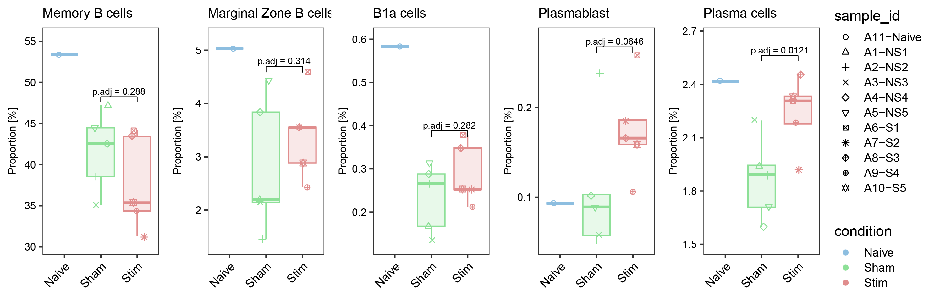
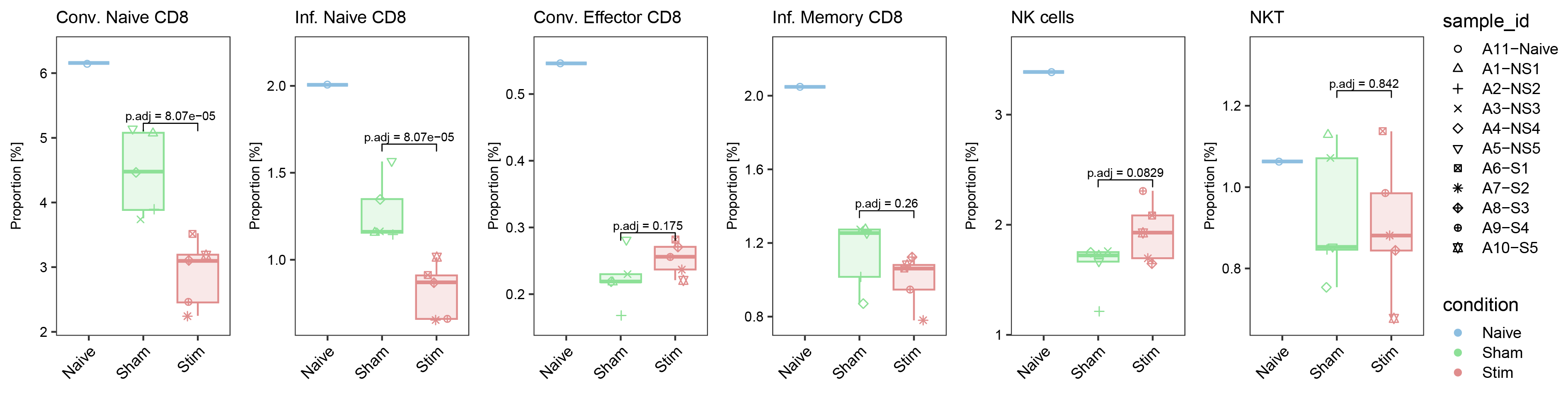
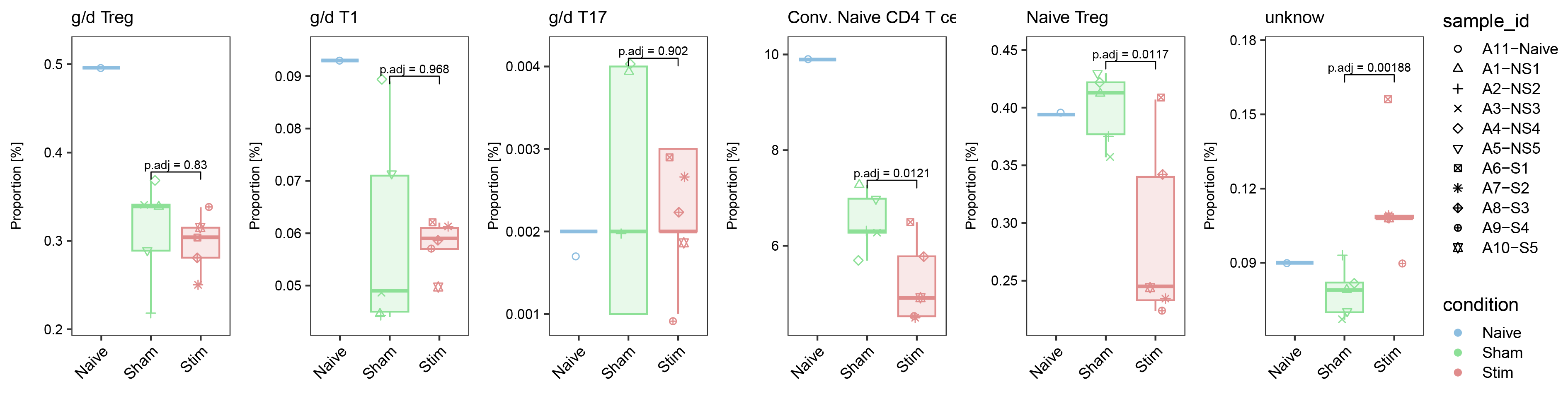
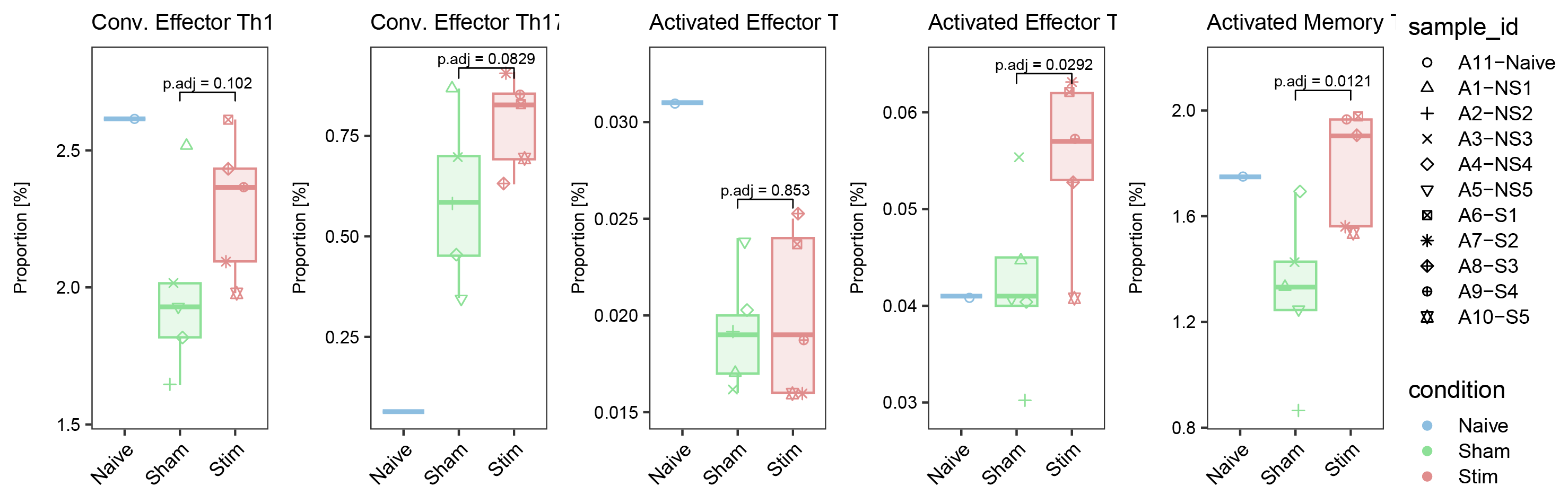
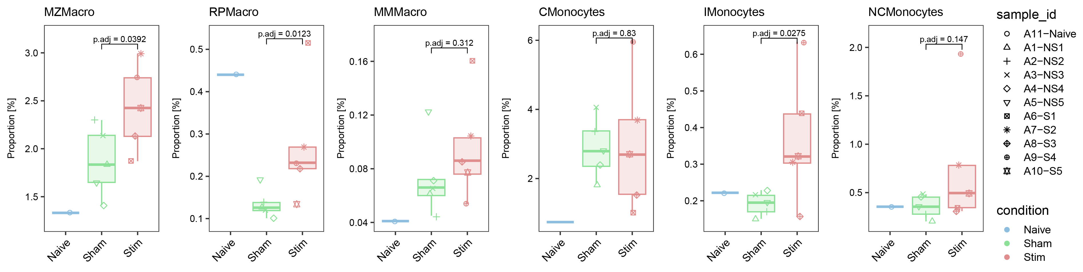
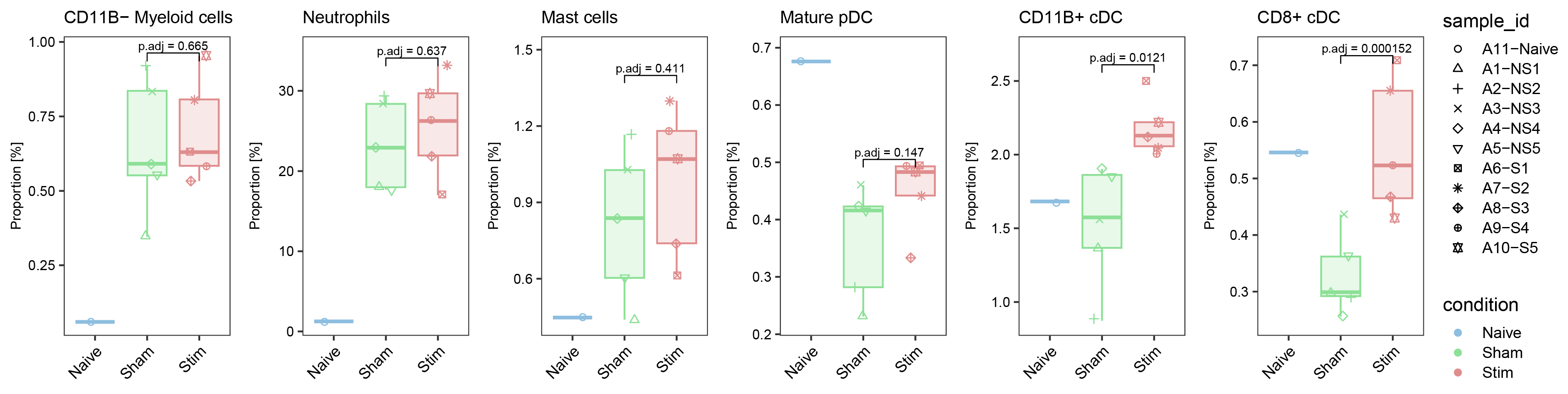
Represent the differential abundances between conditions as boxplots for each group of related subpopulations.

#Boxplots for DA with associated padj 
metadata <- seuratobj@meta.data
metadata = as.data.frame.matrix(table(metadata$sample_id, metadata$celltype))
metadata = as.data.frame(metadata / rowSums(metadata))
metadata$sample_id = rownames(metadata)

metadata = gather(metadata, celltype, percentage, 'Conv. Naive CD8':'unknow')
# metadata$celltype <- factor(metadata$celltype, levels =levels(WangNeurons$celltype_Jung))
metadata$sample_id =factor(metadata$sample_id, levels = c("A11-Naive","A1-NS1" ,"A2-NS2","A3-NS3","A4-NS4","A5-NS5","A6-S1","A7-S2","A8-S3","A9-S4","A10-S5"))

df <- seuratobj@meta.data[,c("sample_id","condition")] %>% unique()
metadata <- inner_join(metadata,df)
metadata$percentage <- round(metadata$percentage*100,digits = 3)


plot_DA_boxplot <- function(metadata,cluster,top_DA){
  meta <- metadata %>% dplyr::filter(celltype%in%c(cluster))
  padj <- top_DA %>% dplyr::filter(cluster_id %in% c(cluster)) %>% pull(p_adj)
  meta2 <- metadata %>% dplyr::filter(celltype%in%c(cluster) & sample_id%ni%c("A11-Naive"))
  ypos <- max(meta2$percentage)+ c(10^floor(log10(max(meta2$percentage)))/10)

  stat.test1 <- tibble(group1=c("Sham"),group2=c("Stim"),p.adj=padj,y.position=ypos)

  p <- ggplot(meta, aes_string(y = "percentage")) +
    labs(x = NULL, y = "Proportion [%]",title = cluster) + 
    theme_bw() + theme(plot.title = element_text(size=10),
                       panel.grid = element_blank(),
                       strip.text = element_text(face = "bold"),
                       strip.background = element_rect(fill = NA, color = NA),
                       axis.text = element_text(color = "black"),
                       axis.text.y = element_text(size = 8),
                       axis.title.y = element_text(size = 8),
                       axis.text.x = element_text(angle = 45, hjust = 1, vjust = 1),
                       legend.key.height  =  unit(0.8, "lines")) + # facet_wrap("celltype", scales = "free_y", ncol = 8) +
    geom_boxplot(aes_string(x = "condition", 
                            color = "condition", fill = "condition"),
                 position = position_dodge(), alpha = 0.2, 
                 outlier.color = NA, show.legend = FALSE) + scale_fill_manual(values=cond.cols) + scale_color_manual(values=cond.cols)+
    geom_point(aes_string(x = "condition", 
                          col = "condition", shape = "sample_id"),
               position = position_jitter(width = 0.2))+ scale_shape_manual(values=1:nlevels(metadata$sample_id))+ scale_fill_manual(values=cond.cols) + scale_color_manual(values=cond.cols)+
    ylim(min(meta$percentage)-c(10^floor(log10(min(meta$percentage)))/10),max(meta$percentage)+ c(10^floor(log10(max(meta$percentage)))/5))
  p + stat_pvalue_manual(stat.test1, size = 2.6,label = "p.adj = {p.adj}")
}

plot_DA_boxplot(metadata=metadata,cluster="Memory B cells",top_DA=top_DA)

list_plot <- list()
for (i in 1:length(levels(sce$celltype))) {
  p1 <- plot_DA_boxplot(metadata=metadata,cluster=levels(sce$celltype)[i],top_DA=top_DA)
  list_plot <- list.append(list_plot,p1)
}
names(list_plot) <- levels(sce$celltype)


ggarrange(list_plot[["Conv. Naive CD8"]],list_plot[["Inf. Naive CD8"]],list_plot[["Conv. Effector CD8"]],list_plot[["Inf. Memory CD8"]],list_plot[["NK cells"]],list_plot[["NKT"]],nrow = 1,ncol = 6,common.legend = T,align = "hv",legend = "right")

ggarrange(list_plot[["g/d Treg"]],list_plot[["g/d T1"]],list_plot[["g/d T17"]],list_plot[["Conv. Naive CD4 T cells"]],list_plot[["Naive Treg"]],list_plot[["unknow"]],nrow = 1,ncol = 6,common.legend = T,align = "hv",legend = "right")

ggarrange(list_plot[["Conv. Effector Th1"]],list_plot[["Conv. Effector Th17"]],list_plot[["Activated Effector T cells"]],list_plot[["Activated Effector Treg"]],list_plot[["Activated Memory Treg"]],nrow = 1,ncol = 5,common.legend = T,align = "hv",legend = "right")

ggarrange(list_plot[["MZMacro"]],list_plot[["RPMacro"]],list_plot[["MMMacro"]],list_plot[["CMonocytes"]],list_plot[["IMonocytes"]],list_plot[["NCMonocytes"]],nrow = 1,ncol = 6,common.legend = T,align = "hv",legend = "right")

ggarrange(list_plot[["CD11B- Myeloid cells"]],list_plot[["Neutrophils"]],list_plot[["Mast cells"]],list_plot[["Mature pDC"]],list_plot[["CD11B+ cDC"]],list_plot[["CD8+ cDC"]],nrow = 1,ncol = 6,common.legend = T,align = "hv",legend = "right")

ggarrange(list_plot[["Memory B cells"]],list_plot[["Marginal Zone B cells"]],list_plot[["B1a cells"]],list_plot[["Plasmablast"]],list_plot[["Plasma cells"]],nrow = 1,ncol = 5,common.legend = T,align = "hv",legend = "right")