Index

Cytometry-high_resolution_clustering

Cytometry Single-cell Secondary Analysis

This module takes pre-processed cytometry data from several samples to run high resolution clustering. The workflow begins by reading protein abundance files (.fcs), which are combined with samples metadata to build a SingleCellExperiment object. After data transformation, quality control checks are performed to ensure data integrity and consistency across samples. The module then applies FlowSOM clustering to identify cell populations, followed by subclustering of specific immune subsets. Each subset undergoes detailed analysis, including 2D visualization techniques, and annotation based on marker intensities.

Module specifications

Input data	Computational environnement	Output data
Flow Cytometry Standard	Cytometry_data_analysis R	annotated data matrices

Code

This module is based on the following documentation :

CyTOF workflow, a suite of R packages to analyse cytometry data
Nowicka M, Krieg C, Crowell HL, Weber LM, Hartmann FJ, Guglietta S, Becher B, Levesque MP, Robinson MD. CyTOF workflow: differential discovery in high-throughput high-dimensional cytometry datasets. F1000Res. 2017 May 26;6:748. doi: 10.12688/f1000research.11622.3.
* https://www.bioconductor.org/packages/release/workflows/vignettes/cytofWorkflow/inst/doc/cytofWorkflow.html#data-import "CyTOF workflow"

This module require to load the following environment of R packages :

source("/data/analysis/data_truchi/Cytometry/ODIN/cytometry_R_packages.R")

Informations about the demo dataset :

The demo dataset results from a standard flow cytometry experiment, containing 5 sham, 5 stimulated samples and 1 naïve sample. Data has been pre-processed in FlowJo.

Notes

This workflow is dedicated to the analysis of already pre-processed data.
Pre-processing steps include removing of dead cells, compensation and checking of marker expression patterns, performed using FlowJo or directly in R.

This workflow can be applied to either fluorescence intensities (flow cytometry) or ion counts (mass cytometry) data.

It combines several R packages dedicated to cytometry data analysis : HDCytoData, flowcore, CATALYST, and diffcyt. It also uses the SingleCellExperiment package to handle protein abundances and cells/channels annotations.

1. Prepare data to build a SingleCellExperiment object containing protein abundances and cells/channels annotations

1.1 Prepare the sample annotation table

A simple annotation table, with ordered condition levels for visualization purposes.

# Import metadata table
md_NH <- read.xlsx("metadata_NH.xlsx")
md_NH$condition <- factor(md_NH$condition,levels = c("Naive","Sham","Stim"))
md_NH$sample_id <- factor(md_NH$sample_id,levels = c("A11-Naive","A1-NS1" ,"A2-NS2","A3-NS3","A4-NS4","A5-NS5","A6-S1","A7-S2","A8-S3","A9-S4","A10-S5"))
md_NH$mice_id <- factor(md_NH$mice_id,levels = c("A11","A1","A2","A3","A4","A5","A6","A7","A8","A9","A10"))
md_NH

1.2 Read the protein abundances files and create a flowset

Protein abundances are stored in .fcs files, pre-processed in FlowJo.

fcs.dir <- c("~/data/")
frames <- lapply(dir(fcs.dir, full.names=TRUE), read.FCS,truncate_max_range = FALSE)
names(frames) <- c("A1-NS1","A10-S5","A11-Naive","A2-NS2","A3-NS3","A4-NS4","A5-NS5","A6-S1","A7-S2","A8-S3","A9-S4")
frames <- frames[c("A11-Naive","A1-NS1","A2-NS2","A3-NS3","A4-NS4","A5-NS5","A6-S1","A7-S2","A8-S3","A9-S4","A10-S5")]

Create a flowset, a set of multiple flowframes.

fs_NH <- as(frames, "flowSet")
fs_NH
sampleNames(fs_NH)

1.3 Read the panel of selected channels

panel_NH <- read.xlsx("cytometry_panel.xlsx")
panel_NH$fcs_colname <- as.character(panel_NH$fcs_colname)
head(data.frame(panel_NH))
# all(panel_NH$fcs_colname %in% colnames(fs_NH))

1.4 Transform the protein abundances data

For mass cytometry data (see the CyTOF workflow vignette) :
* "Usually, the raw marker intensities read by a cytometer have strongly skewed distributions with varying ranges of expression, thus making it difficult to distinguish between the negative and positive cell populations. It is common practice to transform CyTOF marker intensities using, for example, arcsinh (inverse hyperbolic sine) to make the distributions more symmetric and to map them to a comparable range of expression for clustering."
By default, the prepData() SCE constructor arcsinh transforms marker expressions with a cofactor of 5 (5 to 15 is recommended). As the ranges of marker intensities can vary substantially, for visualization, we apply another transformation that scales the expression of all markers to values between 0 and 1 using low (e.g., 1%) and high (e.g., 99%) percentiles as the boundary. This additional transformation of the arcsinh-transformed data can sometimes give better visual representation of relative differences in marker expression between annotated cell populations. However, all computations (differential testing, hierarchical clustering etc.) are still performed on arcsinh-transformed not scaled expressions. Whether scaled expression values should be plotted is specified with argument scale = TRUE or FALSE in the respective visualizations (e.g., plotExprHeatmap() and plotClusterHeatmap())."

For flow cytometry data (see the CytoExploreR vignette https://dillonhammill.github.io/CytoExploreR/articles/CytoExploreR-Transformations.html).
* Multiple transformation possibilities : arcsinh with ajusted cofactor (>100) for each channel, log, biexponential, logicle (similar to biexponential but with less parameters to optimize)

channels <- panel_NH$fcs_colname[which(panel_NH$fcs_colname %in% colnames(fs_NH))]
fs_NH_t <- cyto_transform(fs_NH, type = "logicle",channels= channels,
                          parent = "root",select = c(channels) %>% head(),plot = FALSE,popup = FALSE,display = 25000,axes_limits = "machine")

1.5 Create the SingleCellExperiment object

CATALYST provides the wrapper prepData() to construct a SCE object from the following inputs:
- x: the flowSet containing the measurement data
- panel: the data.frame containing, for each marker, i) its column name in the input raw data, ii) its targeted protein markers, and, optionally, iii) its class (type, state, or none).
- md: the data.frame with columns describing the experimental design.

prepData, by default, checks for non-mass channels and moves them to the int_colData of the output SCE. The reasoning behind this is that all assay data may be subject to data manipulation / computation, e.g., computing quantiles, means, transformations etc. - and this should not happen on categorical variables (e.g. sample IDs, cluster assignments), but only measurement variables (i.e. actual markers). Since there are mass / non-mass channels in FACS (only CyTOF, which CATALYST was built for originally), this behaviour is omitted with FACS = TRUE, which will retain all parameters.

# construct one SingleCellExperiment containing raw data
sce_untransformed <- prepData(fs_NH, panel_NH, md_NH, features = panel_NH$fcs_colname,md_cols = list(file = "file_name", id = "sample_id", factors =c("condition","mice_id")),FACS = TRUE,transform = FALSE)

# construct an other SingleCellExperiment containing raw data
sce <- prepData(fs_NH_t, panel_NH, md_NH, features = panel_NH$fcs_colname,md_cols = list(file = "file_name", id = "sample_id", factors =c("condition","mice_id")),FACS = TRUE,transform = FALSE)
dim(sce)

# create an "exprs" assay, with the normalized data, and a "counts" assay , with the raw data 
sce@assays@data@listData[["exprs"]] <- sce@assays@data@listData[["counts"]]
sce@assays@data@listData[["counts"]] <- sce_untransformed@assays@data@listData[["counts"]]

sce@assays@data@listData[["counts"]][c(10:15),c(10:15)]
sce@assays@data@listData[["exprs"]][c(10:15),c(10:15)]

2. Perform some quality control

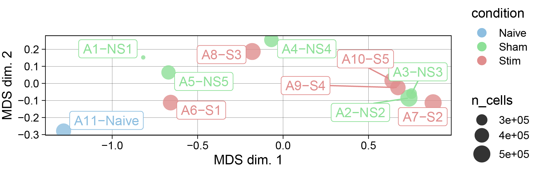
Quick checks to verify whether the data we analyze globally represents what we expect; for example, whether samples that are replicates of one condition are more similar and are distinct from samples from another condition.

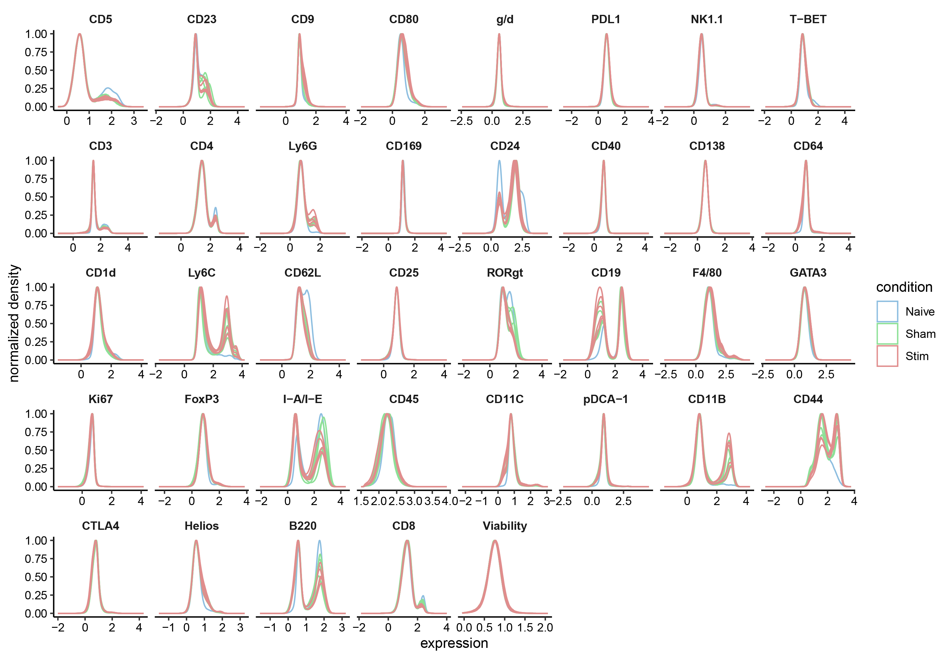
Another important check is to verify that marker expression distributions do not have any abnormalities such as having different ranges or distinct distributions for a subset of the samples. This could highlight problems with the sample collection or data acquisition, or batch effects that were unexpected.

Depending on the situation, one can then consider removing problematic markers or samples from further analysis; in the case of batch effects, a covariate column could be added to the metadata table and used below in the statistical analyses.

cond.cols <- c("Naive"="#8dbee0","Sham"="#8de097","Stim"="#e08d8d")
p <- plotExprs(sce, color_by = "condition",assay="exprs")+scale_color_manual(values=cond.cols)
p$facet$params$ncol <- 8
p

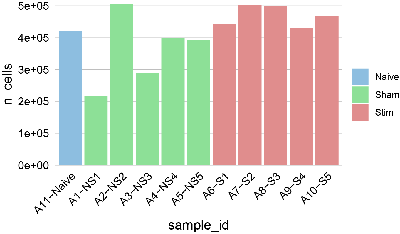
# Check number of cells per sample
n_cells(sce) 
plotCounts(sce, group_by = "sample_id", color_by = "condition")+scale_fill_manual(values=cond.cols)

# MDS plot, a nonlinear dimensionality reduction technique
pbMDS(sce, color_by = "condition", label_by = "sample_id")+scale_color_manual(values=cond.cols)

# Heatmap of median marker intensities with clustered markers and samples
col_fun = colorRamp2(c(0, 0.1,0.2,0.3,0.4,0.5,0.6,0.7,0.8,0.9, 1), rev(hcl.colors(11, "YlGnBu")))
eh <- plotExprHeatmap(sce,by="sample_id",assay = "exprs", scale = "last",hm_pal = rev(hcl.colors(11, "YlGnBu")))
eh@left_annotation@anno_list[["condition"]]@color_mapping@full_col <- cond.cols
eh@left_annotation@anno_list[["condition"]]@fun@var_env[["color_mapping"]]@full_col <- cond.cols
eh

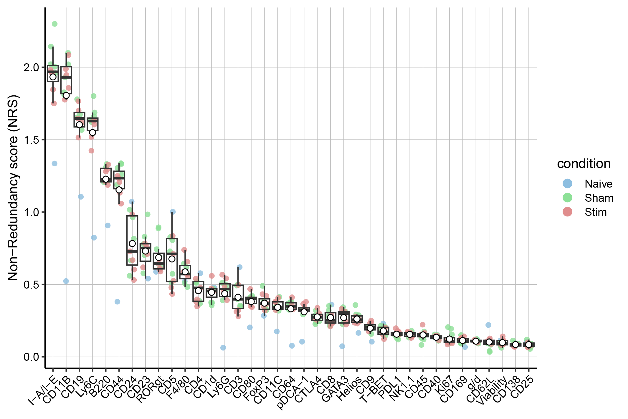
Marker ranking based on the non-redundancy score.
In this step, we identify the ability of markers to explain the variance observed in each sample. In particular, we calculate the PCA-based non-redundancy score (NRS). Markers with higher score explain a larger portion of variability present in a given sample.

The average NRS can be used to select a subset of markers that are non-redundant in each sample but at the same time capture the overall diversity between samples.
Such a subset of markers can then be used for cell population identification analysis (i.e., clustering). We note that there is no precise rule on how to choose the right cutoff for marker inclusion, but one option is to select a suitable number of the top-scoring markers.

The number can be chosen by analyzing the plot with the NR scores, where the markers are sorted by the decreasing average NRS.
Based on prior biological knowledge, one can refine the marker selection and remove markers that are not likely to distinguish cell populations of interest, even if they have high scores, and add in markers with low scores but known to be important in discerning cell subgroups.

plotNRS(sce, features = NULL, color_by = "condition")+scale_color_manual(values=cond.cols)

3. Run the FlowSOM clustering

FlowSOM is among the best performing clustering approaches for cytometry datasets, as it shows strong performance in detecting both high and low frequency cell populations and is one of the fastest methods to run.

The FlowSOM workflow consists of three steps:
1) building a self-organizing map (SOM), where cells are assigned according to their similarities to 100 (by default) grid points (or, so-called codebook vectors or codes) of the SOM
2) building a minimal spanning tree, which is mainly used for graphical representation of the clusters, is skipped in this pipeline
3) metaclustering of the SOM codes, is performed with the ConsensusClusterPlus package. These are wrapped in the CATALYST function cluster(). Additionally, there is an optional round of manual expert-based merging of the metaclusters.

3.1 Clustering on the full dataset

The subset of markers to use for clustering is specified with argument features. For future reference, the specified markers will be assigned class "type", and the remainder of markers will be assigned to be "state" markers. The sets of type and state markers can be accessed at any point with the type_markers() and state_markers() accessor functions, respectively.
Here, we run it on all features.

It's recommended to set max cluster to the maximum of 20, even if it means over-clustering, and manually merge subclusters afterwards.

# for clustering reproductibility, set a stable seed 
set.seed(1234) 
sce <- cluster(sce, features = NULL, xdim = 10, ydim = 10, maxK = 20, seed = 1234)

# Run the UMAP on a subset of cells to increase the speed
set.seed(1234)
sce <- runDR(sce, "UMAP", cells = 1e3, features = NULL) #run on a subset of 1e3 cells per sample
sce <- runDR(sce, "TSNE", cells = 5e3,features = NULL)
sce <- runDR(sce, "PCA", cells = 1e3, features = NULL)

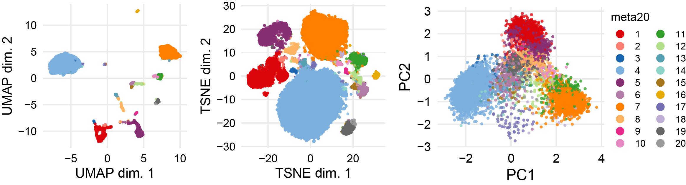
p1 <- plotDR(sce, "UMAP", color_by = "meta20")
p2 <- plotDR(sce, "TSNE", color_by = "meta20")
p3 <- plotDR(sce, "PCA", color_by = "meta20")
ggarrange(p1,p2,p3,ncol=3,nrow = 1,common.legend = T,legend = "right")

# facet by condition
plotDR(sce, "UMAP", color_by = "meta20", facet_by = "condition")


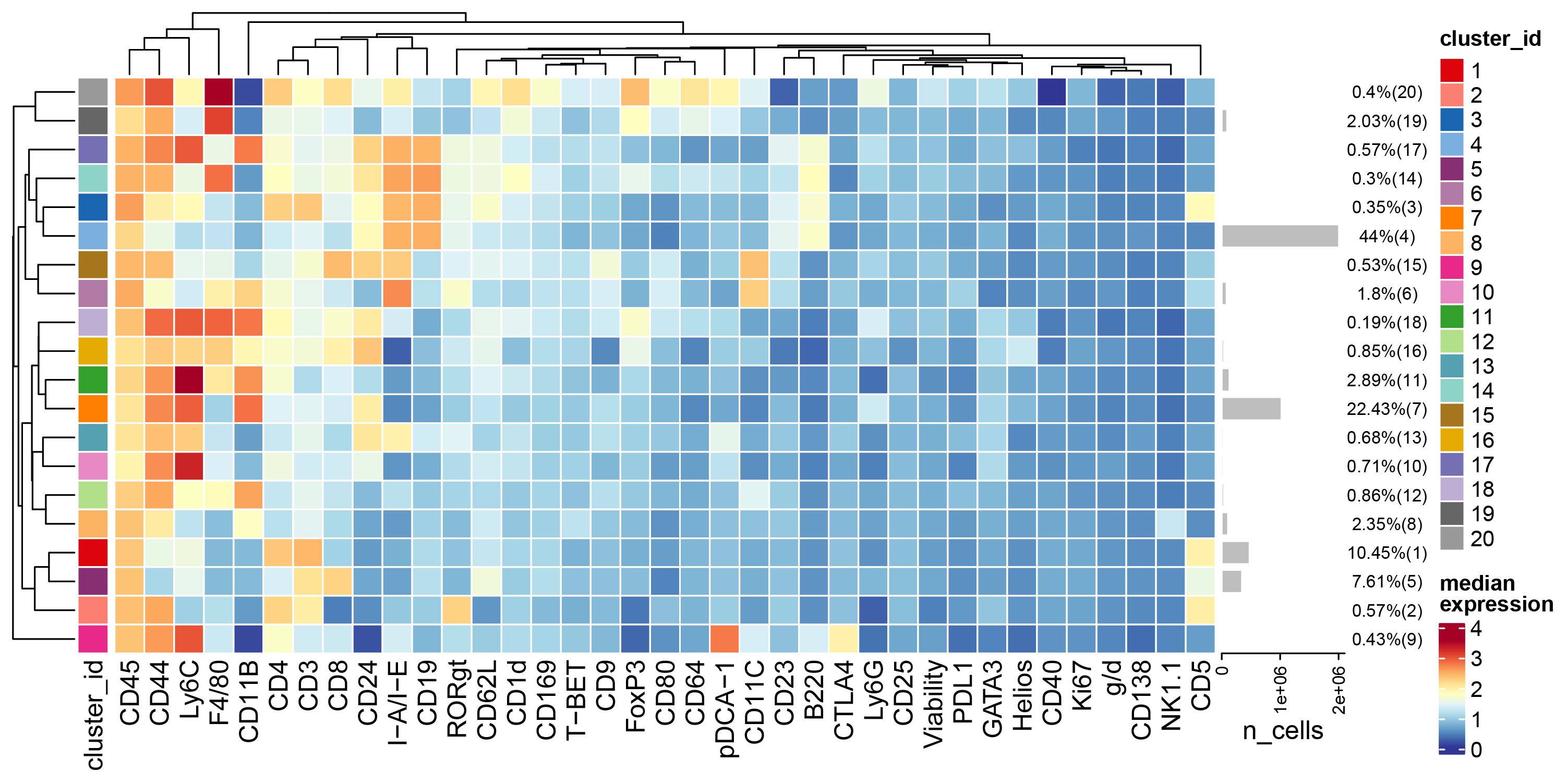
# Heatmap of all markers in all clusters
plotExprHeatmap(sce, features = NULL, by = "cluster_id", k = "meta20", bars = TRUE, perc = TRUE,assay = "exprs",scale = "never")

plotExprHeatmap(sce, features = NULL, by = "cluster_id", k = "meta20", bars = TRUE, perc = TRUE,assay = "exprs",scale = "never",row_clust=FALSE)

# Heatmap of a particular marker intensity in all samples
eh <- plotExprHeatmap(sce, features = "CD11B", by = "both", k = "meta20",assay = "counts",scale = "last", col_clust = FALSE, row_anno = FALSE, bars = FALSE)
eh@top_annotation@anno_list[["condition"]]@color_mapping@full_col <- cond.cols
eh@top_annotation@anno_list[["condition"]]@fun@var_env[["color_mapping"]]@full_col <- cond.cols
eh

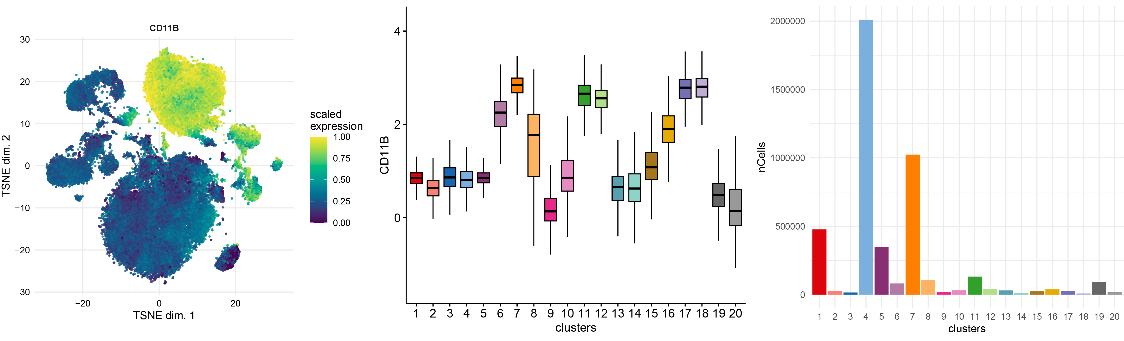
# TSNE of marker expression
p1 <- plotDR(sce, "TSNE", color_by = "CD11B",scale = TRUE,assay = "exprs")

# Boxplot of marker expression per cluster
# add new cluster name to colData
metadata <- sce@metadata[["cluster_codes"]] %>% mutate(cluster_id=som100) %>% dplyr::select(cluster_id,meta20)
metadata2 <- colData(sce) %>% as.data.frame() %>% inner_join(metadata)
sce$clusters <- metadata2$meta20
sce$clusters <- factor(sce$clusters,levels = c("1","2","3","4","5","6","7","8","9","10","11","12","13","14","15","16","17","18","19","20"))

gene <- "CD11B"
cts <- data.frame(counts=sce@assays@data@listData[["exprs"]][gene,])  %>% mutate(clusters=sce$clusters)
p2 <- ggboxplot(cts, x="clusters",y= "counts",fill = "clusters",ylab = gene,palette = CATALYST:::.cluster_cols,outlier.shape = NA)+NoLegend()
p2


# Number of cells per cluster
df <- table(sce$clusters) %>% as.matrix() %>% as.data.frame() %>% mutate(nCells=as.numeric(V1),clusters=rownames(.)) %>% dplyr::select(nCells,clusters)
df$clusters <- factor(df$clusters,levels = c("1","2","3","4","5","6","7","8","9","10","11","12","13","14","15","16","17","18","19","20"))

p3<-ggplot(df, aes(x=clusters, y=nCells, fill=clusters)) +
  geom_bar(stat="identity")+theme_minimal()+scale_fill_manual(values=CATALYST:::.cluster_cols)+NoLegend()
p3

ggarrange(p1,p2,p3,ncol=3,nrow = 1)

3.2 Annotate roughly the clusters

Based on heatmaps of marker expression and biological interest, create a table assigning a cell population to each cluster.

merging_table1 <- read.xlsx("/data/analysis/data_truchi/Cytometry/TS_team_dataset/analysis/clusters20_to_pop.xlsx") %>% dplyr::select("original_cluster","new_cluster")

# convert to factor with merged clusters in desired order
merging_table1$new_cluster <- factor(merging_table1$new_cluster, 
                                     levels = unique(merging_table1$new_cluster))

# apply manual merging 
sce <- mergeClusters(sce, k = "meta20", table = merging_table1, id = "merging1",overwrite = TRUE)

# add new cluster name to colData
metadata <- sce@metadata[["cluster_codes"]] %>% mutate(cluster_id=som100) %>% dplyr::select(cluster_id,merging1)
metadata2 <- colData(sce) %>% as.data.frame() %>% inner_join(metadata)
sce$celltype <- metadata2$merging1
sce$barcode <- paste(sce$condition %>% as.character(), rownames(colData(sce) %>% as.data.frame()),sep = ".")

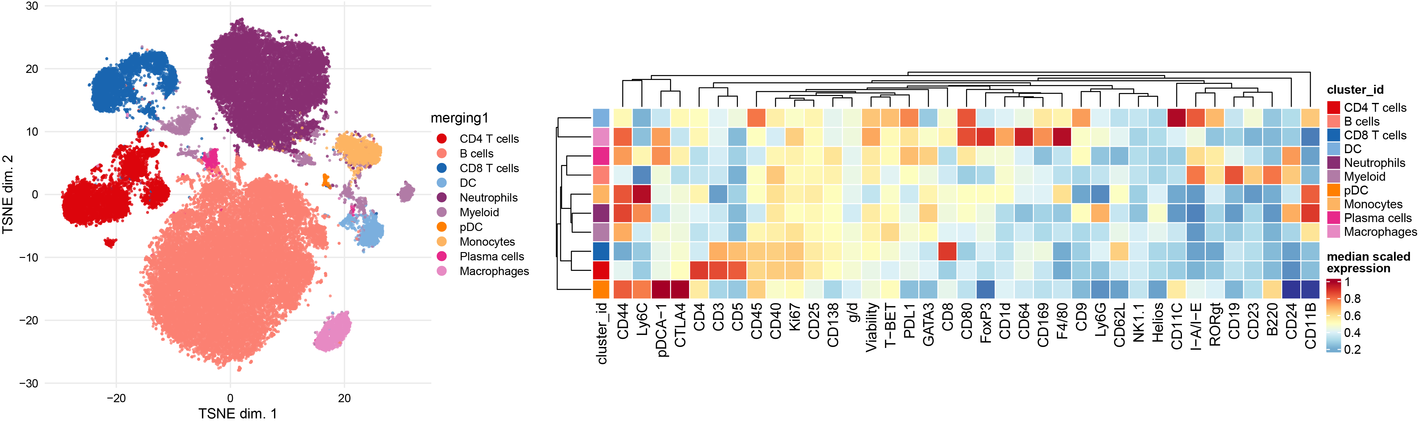
# Plot the coarse annotation
p1 <- plotDR(sce, "TSNE", color_by = "merging1")

# Re-plot the heatmaps based on the coarse annotation
plotExprHeatmap(sce, features = NULL, by = "cluster_id", k = "meta20", m = "merging1")

plotExprHeatmap(sce, features = NULL,by = "cluster_id", k = "merging1")

At this moment, we can save the object as .rds file

saveRDS(sce,file = "cytometry_sce.rds")
sce <- readRDS(file = "cytometry_sce.rds")

3.3 Run subclustering on the distinct immune subsets

Define specific lists of markers that are relevant to identify subpopulations of a particular immune group

CD8.markers <- c("CD11B" ,"CD25","CD3" ,"CD44","CD5" ,"CD62L" ,"CD8" ,"CTLA4" ,"FoxP3","Helios" ,"Ki67", "Ly6C" ,"PDL1","RORgt","T-BET")
CD4.markers <-  c("CD11B" ,"CD25","CD3","CD4","CD44","CD5","CD62L","CTLA4" ,"FoxP3" ,"GATA3","Helios","Ki67", "Ly6C" ,"PDL1","RORgt","T-BET")
B.markers <-c("B220" ,"CD138","CD19","CD1d","CD23","CD24" ,"CD40","CD5","CTLA4" ,"I-A/I-E" , "PDL1" ,"T-BET","CD9","CD80","CD44")
DC.markers <- c("CD11B","CD11C" ,"CD4", "CD40" ,"CD8","CD80" ,"I-A/I-E" ,"Ly6C" ,"pDCA-1")
gd.markers <- c("CD25", "CD3" ,"CD44","CD62L","FoxP3", "g/d" ,"RORgt" ,"T-BET")
NK.markers <- c("CD11B" ,"CD25","CD3" ,"CD4","CD8","FoxP3", "g/d", "GATA3" ,"Ki67" ,"NK1.1","PDL1", "RORgt","T-BET") 
Macro.markers <- c("CD11B","CD169" ,"CD4" ,"CD40" ,"CD64","CD80" ,"F4/80" ,"I-A/I-E","PDL1") 
NeutroMono.markers <- c("CD11B","CD11C" ,"CD24" ,"CD40" ,"CD8", "I-A/I-E","Ly6C" ,"Ly6G" ,"PDL1" ,"T-BET")

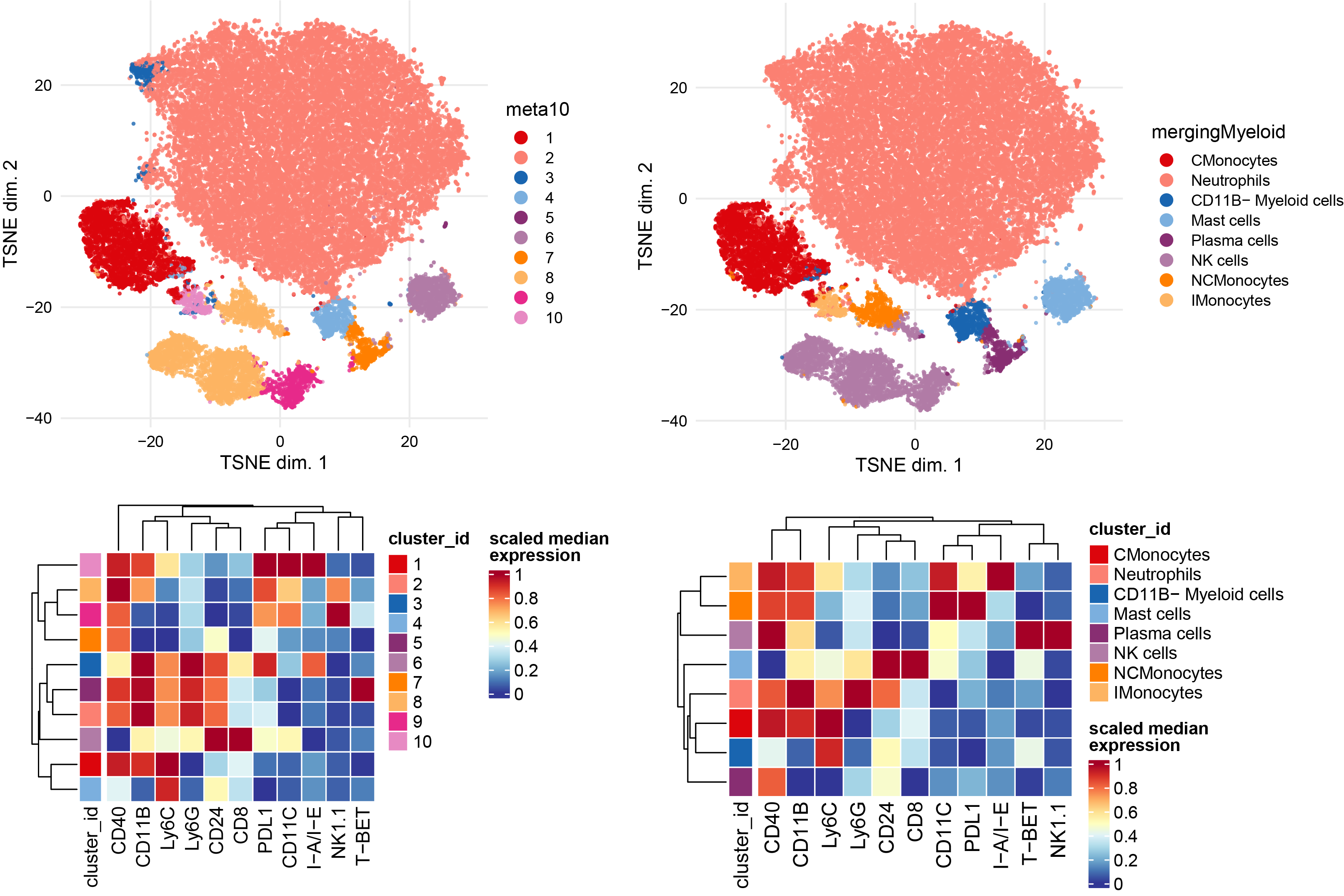
Subclustering of myeloid subset.

# To identify specific myeloid cells, select also monocytes and neutrophils 
Myeloid <- sce[, sce$celltype %in% c("Monocytes","Myeloid","Neutrophils")]
plotDR(Myeloid, "TSNE", color_by = "merging1")

# Run clustering using the selected features
p1 <- plotNRS(Myeloid, features = NULL, color_by = "condition")+scale_color_manual(values=cond.cols)
p1
var.features <- c(NeutroMono.markers,"NK1.1") %>% unique()

# fix a seed for reproducibility
set.seed(1234)
Myeloid <- cluster(Myeloid, features = var.features, xdim = 10, ydim = 10, maxK = 20, seed = 1234) #features = specify which features
p2 <- plotDR(Myeloid, "TSNE", color_by = "meta10")
p2

# Re-run the tSNE 
set.seed(1234)
Myeloid <- runDR(Myeloid, "TSNE", cells = 3e3,features = var.features)
plotDR(Myeloid, "TSNE", color_by = "meta10")

plotDR(Myeloid, "TSNE", color_by = "CD169",scale = TRUE,assay = "exprs")
plotDR(Myeloid, "TSNE", color_by = "CD11C",scale = TRUE,assay = "exprs")
plotDR(Myeloid, "TSNE", color_by = "F4/80",scale = TRUE,assay = "exprs")

# Heatmap of the selected markers intensities per subcluster
plotExprHeatmap(Myeloid, features = var.features, by = "cluster_id", k = "meta10", bars = F, perc = F,assay = "exprs",scale = "last")

# Annotation of subclusters based on markers intensities
newclusts <- c("CMonocytes","Neutrophils","Neutrophils","CD11B- Myeloid cells","Neutrophils","Mast cells","Plasma cells","NK cells","NK cells","NCMonocytes","IMonocytes","Neutrophils")

merging_table_Myeloid <- data.frame(original_cluster=c("1","2","3","4","5","6","7","8","9","10","11","12"),new_cluster=newclusts)
merging_table_Myeloid$new_cluster <- factor(merging_table_Myeloid$new_cluster, 
                                            levels = unique(merging_table_Myeloid$new_cluster))

# apply manual merging
Myeloid <- mergeClusters(Myeloid, k = "meta12", table = merging_table_Myeloid, id = "mergingMyeloid")
plotDR(Myeloid, "TSNE", color_by = "mergingMyeloid")
ggsave("cyto_Myeloid_TSNE_annot.pdf", width = 20, height =10, units = c("cm"), dpi = 300)

plotExprHeatmap(Myeloid, features = c(var.features), by = "cluster_id", k = "mergingMyeloid", bars = F, perc = F,assay = "exprs",scale = "last")

# add new annotation to the colData of the original sce object
metadata <- Myeloid@metadata[["cluster_codes"]] %>% mutate(cluster_id=som100) %>% dplyr::select(cluster_id,mergingMyeloid)
metadata2 <- colData(Myeloid) %>% as.data.frame() %>% inner_join(metadata) %>% mutate(celltype=mergingMyeloid)

df <- as.data.frame(colData(sce))
df <-   setDT(df)[metadata2, celltype := i.celltype , on =.(barcode)]
all(sce$barcode==df$barcode)
sce$celltype <- df$celltype

plotDR(sce, "TSNE", color_by = "celltype")

# Remove the object to save some space
rm(Myeloid)

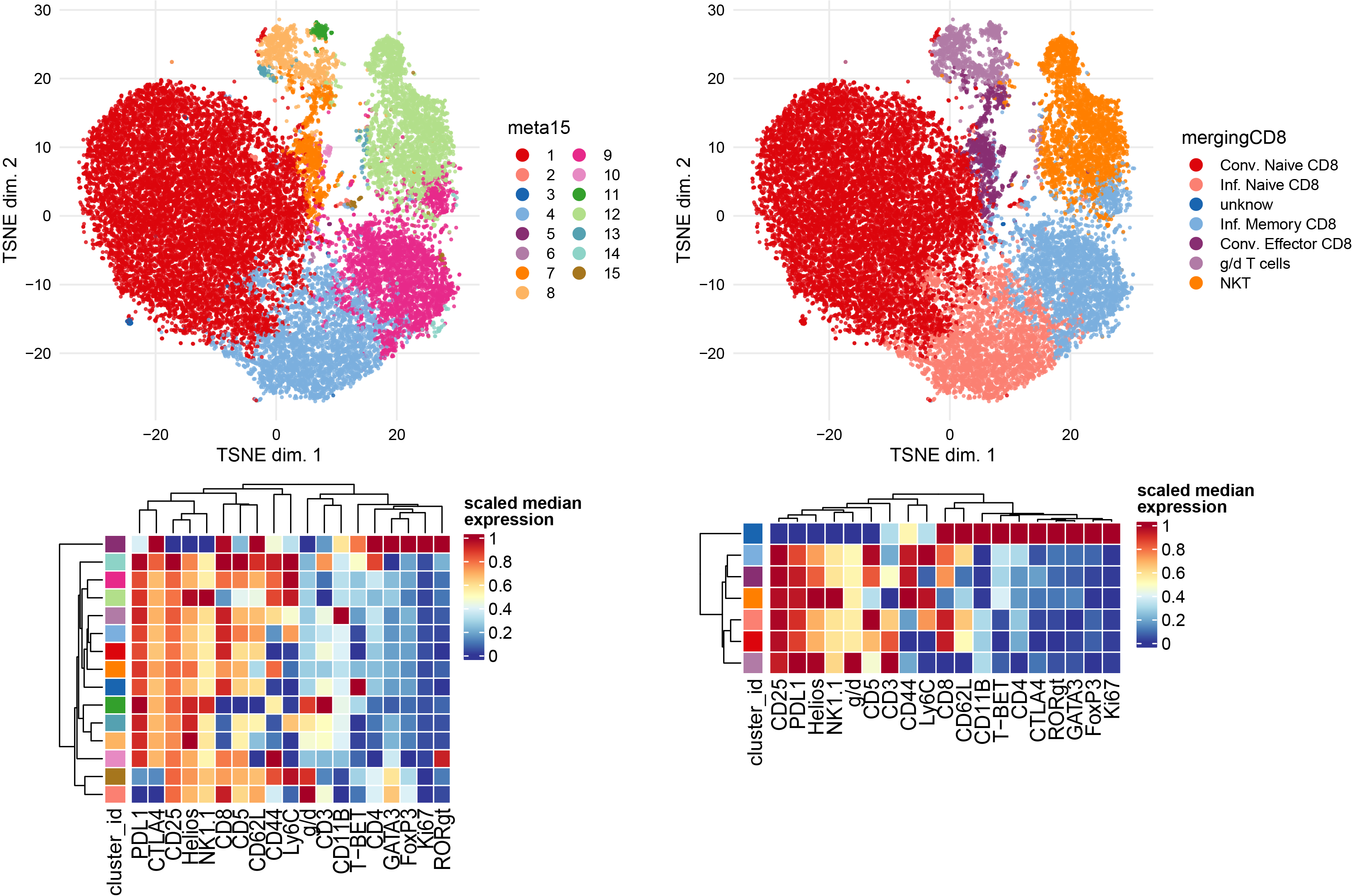
Subclustering of CD8 T cells subset.

CD8 <- sce[, sce$celltype == "CD8 T cells"]
plotDR(CD8, "TSNE", color_by = "celltype")
plotDR(CD8, "TSNE", color_by = "CD44",scale = TRUE,assay = "exprs")

# Run clustering using the selected features
p1 <- plotNRS(CD8, features = NULL, color_by = "condition")+scale_color_manual(values=cond.cols)
p1
var.features <- c(CD8.markers,CD4.markers,gd.markers,NK.markers) %>% unique()

# fix a seed for reproducibility
set.seed(1234)
CD8 <- cluster(CD8, features = var.features, xdim = 10, ydim = 10, maxK = 20, seed = 1234) #features = specify which features

# Re-run the tSNE 
set.seed(1234)
CD8 <- runDR(CD8, "TSNE", cells = 2e3,features = var.features)
plotDR(CD8, "TSNE", color_by = "meta15")
ggsave("cyto_CD8_TSNE_clust.pdf", width = 20, height =10, units = c("cm"), dpi = 300)

# facet by condition
plotDR(CD8, "TSNE", color_by = "CD62L",scale = TRUE,assay = "exprs")
plotDR(CD8, "TSNE", color_by = "CD44",scale = TRUE,assay = "exprs")
plotDR(CD8, "TSNE", color_by = "g/d",scale = TRUE,assay = "exprs")

# Heatmap of the selected markers intensities per subcluster 
plotExprHeatmap(CD8, features = var.features, by = "cluster_id", k = "meta15", bars = F, perc = F,assay = "exprs",scale = "last")


# Annotation of subclusters based on markers intensities 
newclusts <- c("Conv. Naive CD8","Conv. Naive CD8","Conv. Naive CD8","Inf. Naive CD8","unknow","Inf. Memory CD8","Conv. Effector CD8","g/d T cells","Inf. Memory CD8","Conv. Effector CD8","g/d T cells","NKT","g/d T cells","Inf. Memory CD8","Inf. Memory CD8") 
merging_table_CD8 <- data.frame(original_cluster=c("1","2","3","4","5","6","7","8","9","10","11","12","13","14","15"),new_cluster=newclusts)
merging_table_CD8$new_cluster <- factor(merging_table_CD8$new_cluster, 
                                        levels = unique(merging_table_CD8$new_cluster))

# Apply manual merging # add new annotation to the colData of the original sce object
CD8 <- mergeClusters(CD8, k = "meta15", table = merging_table_CD8, id = "mergingCD8")
plotDR(CD8, "TSNE", color_by = "mergingCD8")

plotExprHeatmap(CD8, features = c(var.features,"g/d"), by = "cluster_id", k = "mergingCD8", bars = F, perc = F,assay = "exprs",scale = "last")

# add new cluster name to the colData of the original sce object
metadata <- CD8@metadata[["cluster_codes"]] %>% mutate(cluster_id=som100) %>% dplyr::select(cluster_id,mergingCD8)
metadata2 <- colData(CD8) %>% as.data.frame() %>% inner_join(metadata) %>% mutate(celltype=mergingCD8)

df <- as.data.frame(colData(sce))
df <-   setDT(df)[metadata2, celltype := i.celltype , on =.(barcode)]
all(sce$barcode==df$barcode)
sce$celltype <- df$celltype

plotDR(sce, "TSNE", color_by = "celltype")

# Remove the object to save some space
rm(CD8)

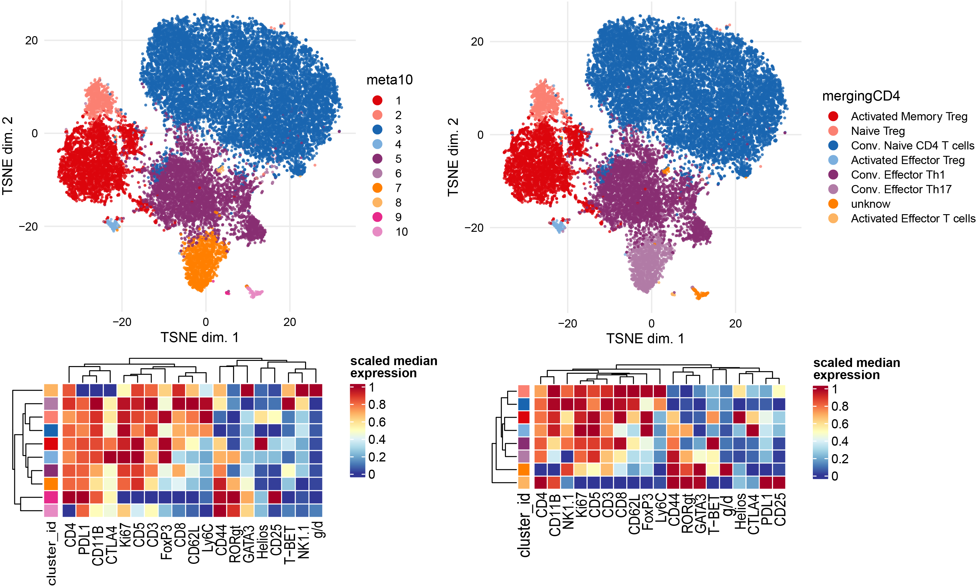
Subclustering of CD4 T cells subset.

CD4 <- sce[, sce$celltype == "CD4 T cells"]
plotDR(CD4, "TSNE", color_by = "merging1")

# Run clustering using the selected features
p1 <- plotNRS(CD4, features = NULL, color_by = "condition")+scale_color_manual(values=cond.cols)
p1
var.features <- c(CD4.markers,CD8.markers,gd.markers,NK.markers) %>% unique()

# fix a seed for reproducibility
set.seed(1234)
CD4 <- cluster(CD4, features = var.features, xdim = 10, ydim = 10, maxK = 20, seed = 1234) #features = specify which features
p2 <-plotDR(CD4, "TSNE", color_by = "meta10")

# Re-run the tSNE 
set.seed(1234)
CD4 <- runDR(CD4, "TSNE", cells = 2e3,features = var.features)
plotDR(CD4, "TSNE", color_by = "meta10")

plotDR(CD4, "TSNE", color_by = "CD62L",scale = TRUE,assay = "exprs")
plotDR(CD4, "TSNE", color_by = "CD44",scale = TRUE,assay = "exprs")
plotDR(CD4, "TSNE", color_by = "CD25",scale = TRUE,assay = "exprs")
plotDR(CD4, "TSNE", color_by = "FoxP3",scale = TRUE,assay = "exprs")
plotDR(CD4, "TSNE", color_by = "CTLA4",scale = TRUE,assay = "exprs")
plotDR(CD4, "TSNE", color_by = "RORgt",scale = TRUE,assay = "exprs")
plotDR(CD4, "TSNE", color_by = "GATA3",scale = TRUE,assay = "exprs")
plotDR(CD4, "TSNE", color_by = "T-BET",scale = TRUE,assay = "exprs")

# Heatmap of the selected markers intensities per subcluster
plotExprHeatmap(CD4, features = var.features, by = "cluster_id", k = "meta10", bars = F, perc = F,assay = "exprs",scale = "last")

newclusts <- c("Activated Memory Treg","Naive Treg","Conv. Naive CD4 T cells","Activated Effector Treg","Conv. Effector Th1","Conv. Naive CD4 T cells","Conv. Effector Th17","unknow","Activated Effector T cells","unknow")

# Annotation of subclusters based on markers intensities 
merging_table_CD4 <- data.frame(original_cluster=c("1","2","3","4","5","6","7","8","9","10"),new_cluster=newclusts)
merging_table_CD4$new_cluster <- factor(merging_table_CD4$new_cluster, 
                                        levels = unique(merging_table_CD4$new_cluster))

# Apply manual merging # add new annotation to the colData of the original sce object
CD4 <- mergeClusters(CD4, k = "meta10", table = merging_table_CD4, id = "mergingCD4")
plotDR(CD4, "TSNE", color_by = "mergingCD4")

plotExprHeatmap(CD4, features = c(var.features), by = "cluster_id", k = "mergingCD4", bars = F, perc = F,assay = "exprs",scale = "last")

# Add new cluster name to the colData of the original sce object
metadata <- CD4@metadata[["cluster_codes"]] %>% mutate(cluster_id=som100) %>% dplyr::select(cluster_id,mergingCD4)
metadata2 <- colData(CD4) %>% as.data.frame() %>% inner_join(metadata) %>% mutate(celltype=mergingCD4)

df <- as.data.frame(colData(sce))
df <-   setDT(df)[metadata2, celltype := i.celltype , on =.(barcode)]
all(sce$barcode==df$barcode)
sce$celltype <- df$celltype

plotDR(sce, "TSNE", color_by = "celltype")

# Remove the object to save some space
rm(CD4)

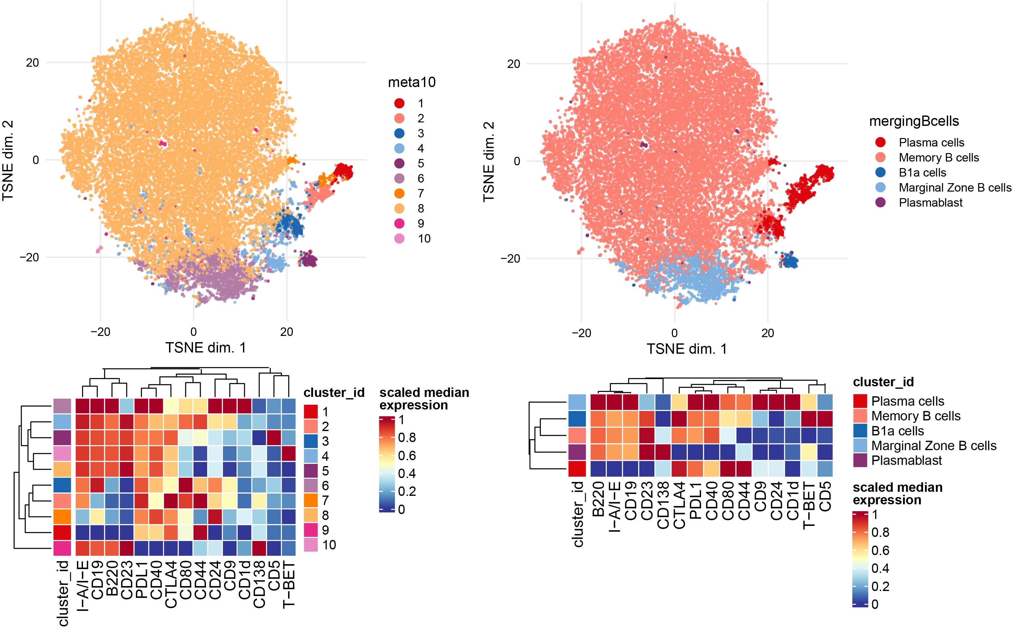
Subclustering of B cells subset.

Bcells <- sce[, sce$celltype %in% c("B cells","Plasma cells")]
plotDR(Bcells, "TSNE", color_by = "merging1")

# Run clustering using the selected features
p1 <- plotNRS(Bcells, features = NULL, color_by = "condition")+scale_color_manual(values=cond.cols)
p1
var.features <- c(B.markers) %>% unique()

# fix a seed for reproducibility
set.seed(1234) 
Bcells <- cluster(Bcells, features = var.features, xdim = 10, ydim = 10, maxK = 20, seed = 1234) #features = specify which features

# Re-run the tSNE 
set.seed(1234)
Bcells <- runDR(Bcells, "TSNE", cells = 2e3,features = var.features)
plotDR(Bcells, "TSNE", color_by = "meta10")

ggarrange(
  plotDR(Bcells, "TSNE", color_by = "B220",scale = TRUE,assay = "exprs"),
  plotDR(Bcells, "TSNE", color_by = "CD138",scale = TRUE,assay = "exprs"),
  plotDR(Bcells, "TSNE", color_by = "CD44",scale = TRUE,assay = "exprs"),
  plotDR(Bcells, "TSNE", color_by = "CD44",scale = TRUE,assay = "exprs"),
  plotDR(Bcells, "TSNE", color_by = "CD1d",scale = TRUE,assay = "exprs"),
  plotDR(Bcells, "TSNE", color_by = "CD23",scale = TRUE,assay = "exprs"),
  plotDR(Bcells, "TSNE", color_by = "CD44",scale = TRUE,assay = "exprs"),
  plotDR(Bcells, "TSNE", color_by = "CD24",scale = TRUE,assay = "exprs"),
  plotDR(Bcells, "TSNE", color_by = "CD5",scale = TRUE,assay = "exprs"),ncol=3,nrow=3)

# Heatmap of the selected markers intensities per subcluster 
plotExprHeatmap(Bcells, features = var.features, by = "cluster_id", k = "meta10", bars = F, perc = F,assay = "exprs",scale = "last")


# Annotation of subclusters based on markers intensities 
newclusts <- c("Plasma cells","Plasma cells","Plasma cells","Memory B cells","B1a cells","Marginal Zone B cells","Plasma cells","Memory B cells","Plasmablast","Memory B cells")

merging_table_Bcells <- data.frame(original_cluster=c("1","2","3","4","5","6","7","8","9","10"),new_cluster=newclusts)
merging_table_Bcells$new_cluster <- factor(merging_table_Bcells$new_cluster, 
                                           levels = unique(merging_table_Bcells$new_cluster))

# Apply manual merging # add new annotation to the colData of the original sce object
Bcells <- mergeClusters(Bcells, k = "meta10", table = merging_table_Bcells, id = "mergingBcells")
plotDR(Bcells, "TSNE", color_by = "mergingBcells")

plotExprHeatmap(Bcells, features = c(var.features), by = "cluster_id", k = "mergingBcells", bars = F, perc = F,assay = "exprs",scale = "last")

# add new cluster name to the colData of the original sce object
metadata <- Bcells@metadata[["cluster_codes"]] %>% mutate(cluster_id=som100) %>% dplyr::select(cluster_id,mergingBcells)
metadata2 <- colData(Bcells) %>% as.data.frame() %>% inner_join(metadata) %>% mutate(celltype=mergingBcells)

df <- as.data.frame(colData(sce))
df <-   setDT(df)[metadata2, celltype := i.celltype , on =.(barcode)]
all(sce$barcode==df$barcode)
sce$celltype <- df$celltype

plotDR(sce, "TSNE", color_by = "celltype")

# Remove the object to save some space
rm(Bcells)

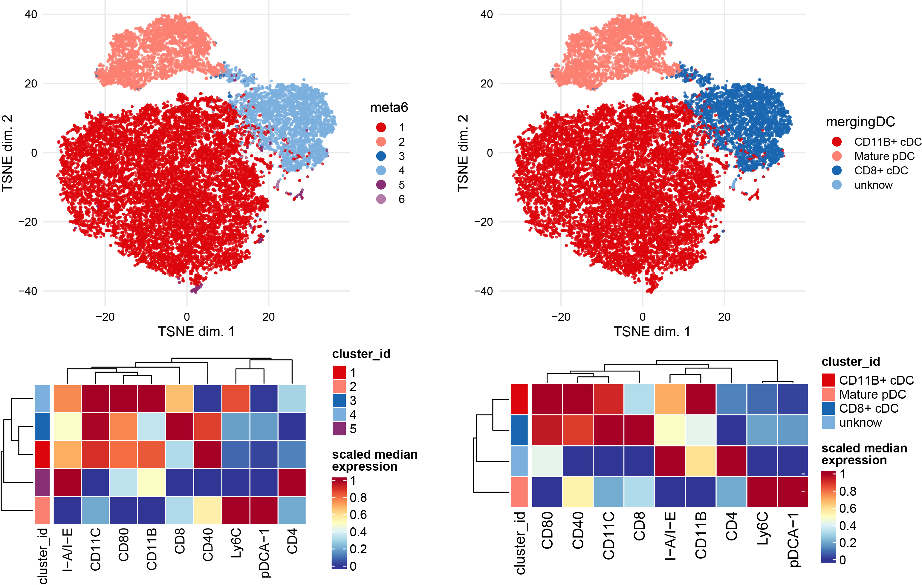
Subclustering of DC subset.

DC <- sce[, sce$celltype %in% c("DC","pDC")]
plotDR(DC, "TSNE", color_by = "merging1")

# Run clustering using the selected features
p1 <- plotNRS(DC, features = NULL, color_by = "condition")+scale_color_manual(values=cond.cols)
p1
var.features <- c(DC.markers) %>% unique()

# fix a seed for reproducibility
set.seed(1234)
DC <- cluster(DC, features = var.features, xdim = 10, ydim = 10, maxK = 20, seed = 1234) #features = specify which features
p2 <-plotDR(DC, "TSNE", color_by = "meta10")

# Re-run the tSNE 
set.seed(1234)
DC <- runDR(DC, "TSNE", cells = 2e3,features = var.features)
plotDR(DC, "TSNE", color_by = "meta6")

plotDR(DC, "TSNE", color_by = "B220",scale = TRUE,assay = "exprs")
plotDR(DC, "TSNE", color_by = "I-A/I-E",scale = TRUE,assay = "exprs")
plotDR(DC, "TSNE", color_by = "Ly6C",scale = TRUE,assay = "exprs")

# Heatmap of the selected markers intensities per subcluster
plotExprHeatmap(DC, features = var.features, by = "cluster_id", k = "meta5", bars = F, perc = F,assay = "exprs",scale = "last")

# Annotation of subclusters based on markers intensities 
newclusts <- c("CD11B+ cDC","Mature pDC","CD8+ cDC","CD11B+ cDC","unknow")

merging_table_DC <- data.frame(original_cluster=c("1","2","3","4","5"),new_cluster=newclusts)
merging_table_DC$new_cluster <- factor(merging_table_DC$new_cluster, 
                                       levels = unique(merging_table_DC$new_cluster))

# Apply manual merging # add new annotation to the colData of the original sce object
DC <- mergeClusters(DC, k = "meta5", table = merging_table_DC, id = "mergingDC")
plotDR(DC, "TSNE", color_by = "mergingDC")

plotExprHeatmap(DC, features = c(var.features), by = "cluster_id", k = "mergingDC", bars = F, perc = F,assay = "exprs",scale = "last")

# add new cluster name to the colData of the original sce object
metadata <- DC@metadata[["cluster_codes"]] %>% mutate(cluster_id=som100) %>% dplyr::select(cluster_id,mergingDC)
metadata2 <- colData(DC) %>% as.data.frame() %>% inner_join(metadata) %>% mutate(celltype=mergingDC)

df <- as.data.frame(colData(sce))
df <-   setDT(df)[metadata2, celltype := i.celltype , on =.(barcode)]
all(sce$barcode==df$barcode)
sce$celltype <- df$celltype

plotDR(sce, "TSNE", color_by = "celltype")

# Remove the object to save some space
rm(DC)

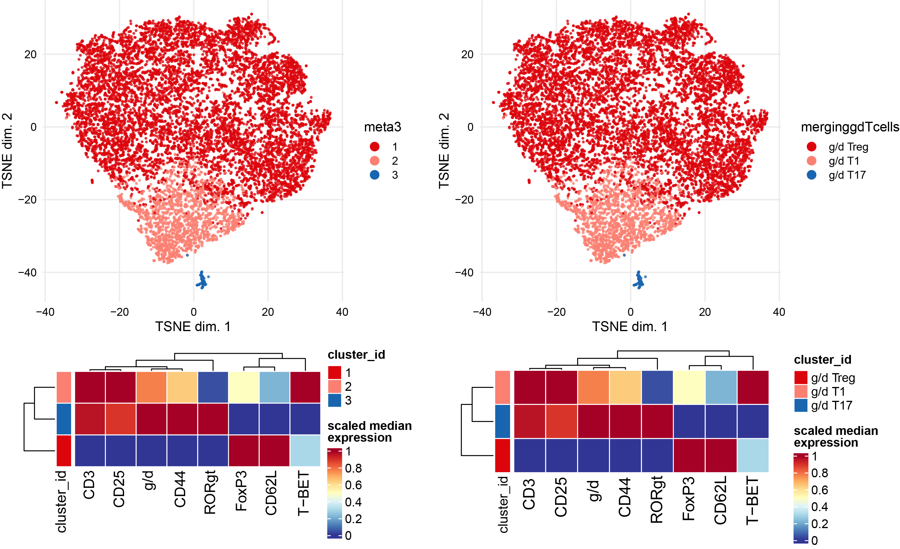
Subclustering of gdTcells subset.

gdTcells <- sce[, sce$celltype %in% c("g/d T cells")]
plotDR(gdTcells, "TSNE", color_by = "merging1")

## Run clustering using the selected features
p1 <- plotNRS(gdTcells, features = NULL, color_by = "condition")+scale_color_manual(values=cond.cols)
p1
var.features <- c(gd.markers) %>% unique()

# fix a seed for reproducibility
set.seed(1234) 
gdTcells <- cluster(gdTcells, features = var.features, xdim = 10, ydim = 10, maxK = 20, seed = 1234) #features = specify which features
plotDR(gdTcells, "TSNE", color_by = "meta10")

# Re-run the tSNE 
set.seed(1234)
gdTcells <- runDR(gdTcells, "TSNE", cells = 1e3,features = var.features)
plotDR(gdTcells, "TSNE", color_by = "meta3")

ggarrange(
  plotDR(gdTcells, "TSNE", color_by = "T-BET",scale = TRUE,assay = "exprs"),
  plotDR(gdTcells, "TSNE", color_by = "RORgt",scale = TRUE,assay = "exprs"),
  plotDR(gdTcells, "TSNE", color_by = "FoxP3",scale = TRUE,assay = "exprs"))

# Heatmap of the selected markers intensities per subcluster  
plotExprHeatmap(gdTcells, features = var.features, by = "cluster_id", k = "meta3", bars = F, perc = F,assay = "exprs",scale = "last")

# Annotation of subclusters based on markers intensities 
newclusts <- c("g/d Treg" ,"g/d T1","g/d T17")

merging_table_gdTcells <- data.frame(original_cluster=c("1","2","3"),new_cluster=newclusts)
merging_table_gdTcells$new_cluster <- factor(merging_table_gdTcells$new_cluster, 
                                             levels = unique(merging_table_gdTcells$new_cluster))

# Apply manual merging # add new annotation to the colData of the original sce object
gdTcells <- mergeClusters(gdTcells, k = "meta3", table = merging_table_gdTcells, id = "merginggdTcells",overwrite = T)
plotDR(gdTcells, "TSNE", color_by = "merginggdTcells")

plotExprHeatmap(gdTcells, features = c(var.features), by = "cluster_id", k = "merginggdTcells", bars = F, perc = F,assay = "exprs",scale = "last")

# add new cluster name to the colData of the original sce object
metadata <- gdTcells@metadata[["cluster_codes"]] %>% mutate(cluster_id=som100) %>% dplyr::select(cluster_id,merginggdTcells)
metadata2 <- colData(gdTcells) %>% as.data.frame() %>% inner_join(metadata) %>% mutate(celltype=merginggdTcells)

df <- as.data.frame(colData(sce))
df <-   setDT(df)[metadata2, celltype := i.celltype , on =.(barcode)]
all(sce$barcode==df$barcode)
sce$celltype <- df$celltype

plotDR(sce, "TSNE", color_by = "celltype")

# Remove the object to save some space
rm(gdTcells)

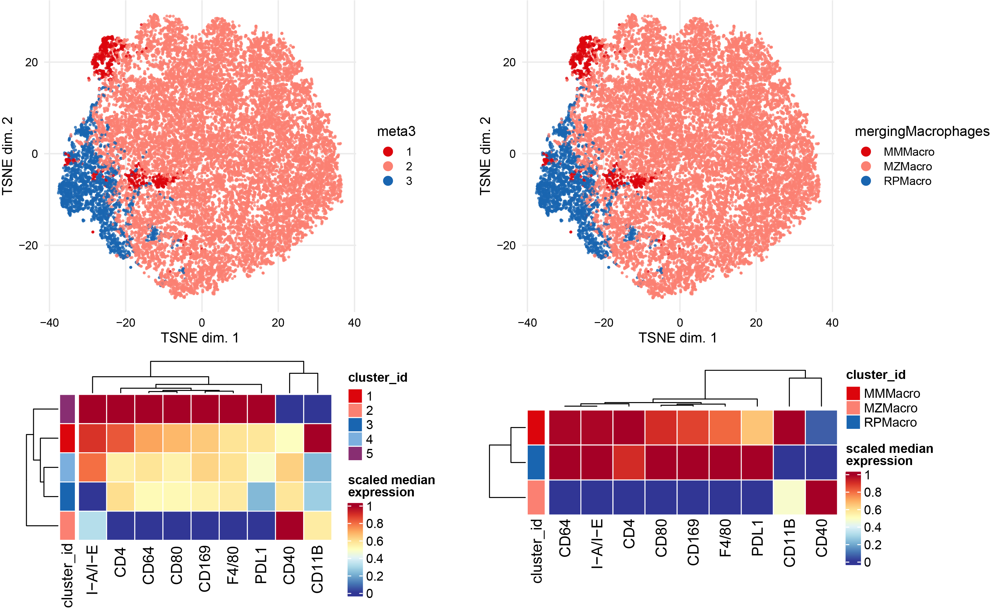
Subclustering of Macrophages subset.

Macrophages <- sce[, sce$celltype %in% c("Macrophages")]
plotDR(Macrophages, "TSNE", color_by = "merging1")

# Run clustering using the selected features
p1 <- plotNRS(Macrophages, features = NULL, color_by = "condition")+scale_color_manual(values=cond.cols)
p1
var.features <- c(Macro.markers) %>% unique()

# fix a seed for reproducibility
set.seed(1234)
Macrophages <- cluster(Macrophages, features = var.features, xdim = 10, ydim = 10, maxK = 20, seed = 1234) #features = specify which features
plotDR(Macrophages, "TSNE", color_by = "meta3")

# Re-run the tSNE 
set.seed(1234)
Macrophages <- runDR(Macrophages, "TSNE", cells = 2e3,features = var.features)
plotDR(Macrophages, "TSNE", color_by = "meta3")

ggarrange(
  plotDR(Macrophages, "TSNE", color_by = "CD169",scale = TRUE,assay = "exprs"),
  plotDR(Macrophages, "TSNE", color_by = "CD11B",scale = TRUE,assay = "exprs"),
  plotDR(Macrophages, "TSNE", color_by = "F4/80",scale = TRUE,assay = "exprs"))

# Heatmap of the selected markers intensities per subcluster  
plotExprHeatmap(Macrophages, features = var.features, by = "cluster_id", k = "meta5", bars = F, perc = F,assay = "exprs",scale = "last")

# Annotation of subclusters based on markers intensities 
newclusts <- c("MMMacro","MZMacro","RPMacro")
merging_table_Macrophages <- data.frame(original_cluster=c("1","2","3"),new_cluster=newclusts)
merging_table_Macrophages$new_cluster <- factor(merging_table_Macrophages$new_cluster, 
                                                levels = unique(merging_table_Macrophages$new_cluster))

# Apply manual merging # add new annotation to the colData of the original sce object
Macrophages <- mergeClusters(Macrophages, k = "meta3", table = merging_table_Macrophages, id = "mergingMacrophages")
plotDR(Macrophages, "TSNE", color_by = "mergingMacrophages")

plotExprHeatmap(Macrophages, features = c(var.features), by = "cluster_id", k = "mergingMacrophages", bars = F, perc = F,assay = "exprs",scale = "last")

# add new cluster name to the colData of the original sce object
metadata <- Macrophages@metadata[["cluster_codes"]] %>% mutate(cluster_id=som100) %>% dplyr::select(cluster_id,mergingMacrophages)
metadata2 <- colData(Macrophages) %>% as.data.frame() %>% inner_join(metadata) %>% mutate(celltype=mergingMacrophages)

df <- as.data.frame(colData(sce))
df <-   setDT(df)[metadata2, celltype := i.celltype , on =.(barcode)]
all(sce$barcode==df$barcode)
sce$celltype <- df$celltype

plotDR(sce, "TSNE", color_by = "celltype")

# Remove the object to save some space
rm(Macrophages)

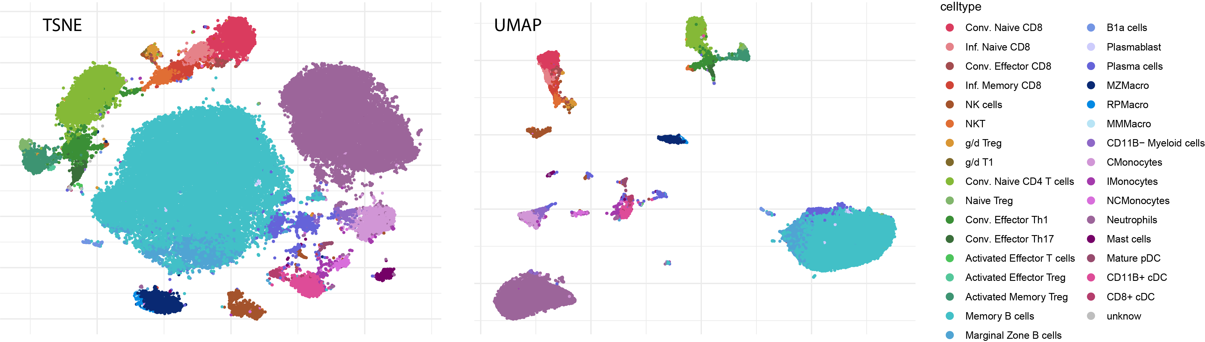
3.4 Plot the main representations with the refined annotation

Save the final object with the refined annotation

saveRDS(sce,file = "cytometry_sce.rds")
sce <- readRDS("cytometry_sce.rds")

Plot the refined annotation after re-running tSNE and UMAP on selected markers.

colors.NH <- c("Conv. Naive CD8"="#da3b5e","Inf. Naive CD8"="#e58289","Conv. Effector CD8"="#a34c4f","Inf. Memory CD8"="#d04336","NK cells"="#a4532b","NKT"= "#e06e34","g/d Treg"="#d99634","g/d T1"="#806a2b","g/d T17"="#bdb02e","Conv. Naive CD4 T cells"="#85b937","Naive Treg"="#81b66c","Conv. Effector Th1"="#3a8f36","Conv. Effector Th17"="#3a6e3a","Activated Effector T cells"="#4cc45b","Activated Effector Treg"="#54c79a","Activated Memory Treg"="#3d9472",
               "Memory B cells"="#42c0c7","Marginal Zone B cells"="#50a4d3","B1a cells"="#7395e4","Plasmablast"="#cdccfc","Plasma cells"="#6563d9",
               "MZMacro"="#092973","RPMacro"="#0289e3","MMMacro"="#b8e4f5",
               "CD11B- Myeloid cells"="#8e68c7","CMonocytes"="#d196d6","IMonocytes"="#a43aac","NCMonocytes"="#d86edb","Neutrophils"="#9c659a","Mast cells"="#750067","Mature pDC"="#974b6d","CD11B+ cDC"="#de4c98","CD8+ cDC"="#b53d6c","unknow"="grey")

sce$celltype <- factor(as.character(sce$celltype),levels = names(colors.NH))

features_rd <- c(CD8.markers,CD4.markers,B.markers,DC.markers,gd.markers,NK.markers,Macro.markers,NeutroMono.markers) %>% unique()

set.seed(1)
sce <- runDR(sce, "TSNE", cells = 5e3, features = features_rd)

set.seed(1)
sce <- runDR(sce, "UMAP", cells = 5e3, features = features_rd) 

p <-plotDR(sce, "TSNE", color_by = "celltype")
p1 <- p[["data"]]
p1 <- inner_join(p1,data.frame(celltype=names(colors.NH),color=colors.NH))
p1$celltype <- factor(as.character(p1$celltype),levels = names(colors.NH))

pTSNE <- ggplot(p1, aes(x=x, y=y, color=celltype)) + 
  geom_point(size = 0.5)+scale_color_manual(values=colors.NH)+theme_minimal() +
  theme(axis.text.x = element_blank(),
        axis.title.y = element_blank(),
        axis.title.x = element_blank(),
        axis.text.y = element_blank())
pTSNE+NoLegend()
# ggsave("TSNE_celltypes.pdf",height = 10,width = 10)

p <-plotDR(sce, "UMAP", color_by = "celltype")
p1 <- p[["data"]]
p1 <- inner_join(p1,data.frame(celltype=names(colors.NH),color=colors.NH))
p1$celltype <- factor(as.character(p1$celltype),levels = names(colors.NH))

pUMAP <-ggplot(p1, aes(x=x, y=y, color=celltype)) + 
  geom_point(size = 0.5)+scale_color_manual(values=colors.NH)+theme_minimal() +
  theme(axis.text.x = element_blank(),
        axis.title.y = element_blank(),
        axis.title.x = element_blank(),
        axis.text.y = element_blank())
pUMAP+NoLegend()
ggarrange(pTSNE,pUMAP,ncol=2,nrow=1,common.legend=TRUE,legend="right")

Plot the refined annotation after re-running tSNE and UMAP on selected markers.

#  Transform into seurat object
# Seurat is the most popular packages to handle and analyze single-cell RNA-seq 
data <- sce@assays@data@listData[["exprs"]]
data <- as(data,"dgCMatrix")
metadata <- colData(sce) %>% as.data.frame()
rownames(metadata) <- metadata$barcode
colnames(data) <- metadata$barcode
seuratobj <- CreateSeuratObject(counts = data,meta.data = metadata,min.cells = 0,min.features = 0)

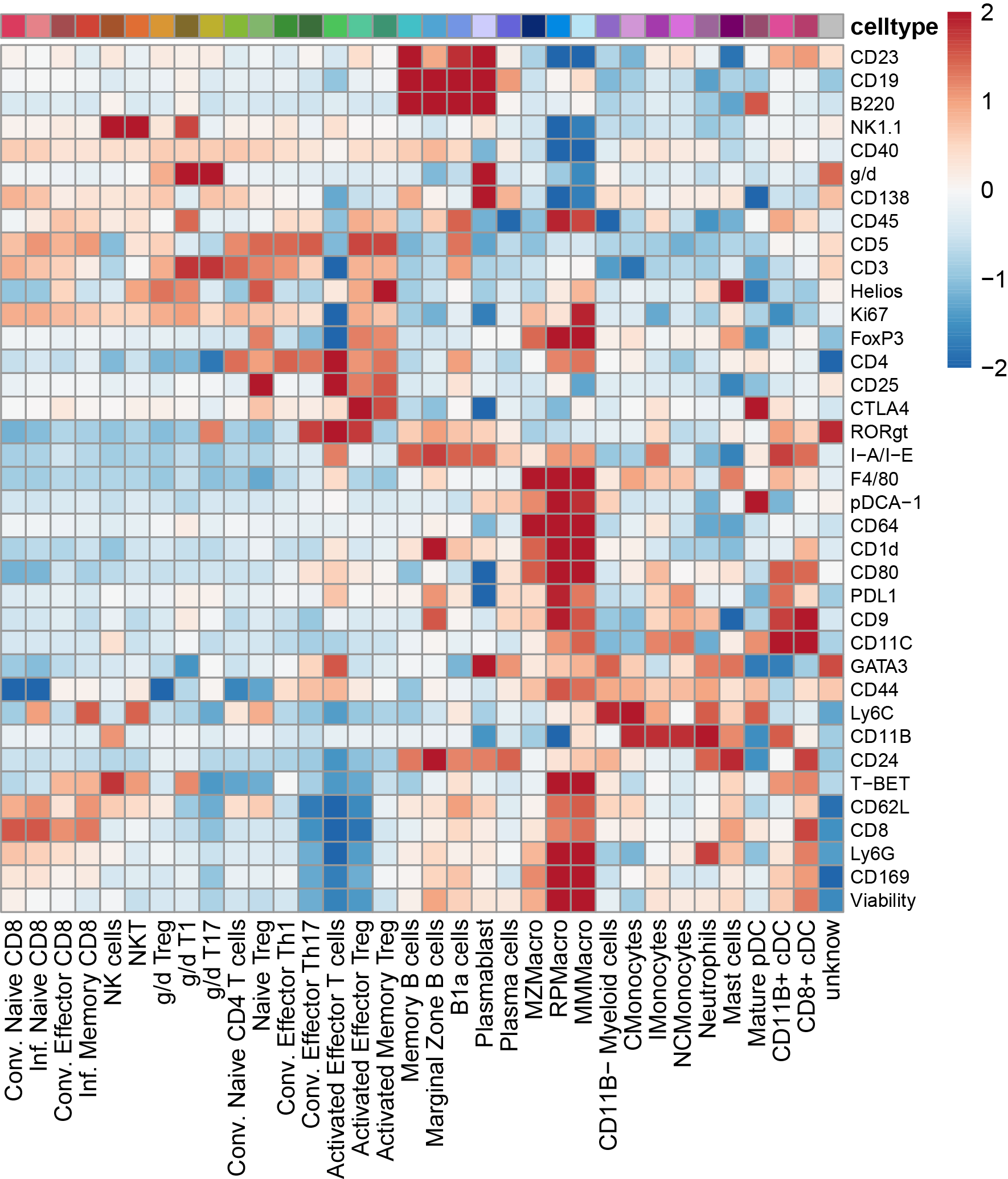
# Heatmap of markers expression in refined clustering
Idents(seuratobj) <- "celltype"
average <- AverageExpression(seuratobj, return.seurat = T,layer = "counts")

data <- GetAssayData(average,layer = "data")
annotation <- data.frame(row.names =colnames(data),celltype=colnames(data))
# annotation$celltype <- factor(annotation$celltype,levels = celltype.order)
data <- flexible_normalization(data)
data[data < -2] <- -2
data[data > 2] <- 2


paletteLength = 100
myColor = colorRampPalette(rev(brewer.pal(n = 9, name ="RdBu")))(paletteLength)
Breaks = c(seq(min(data), 0, length.out=ceiling(paletteLength/2) + 1),
           seq(max(data)/paletteLength, max(data), length.out=floor(paletteLength/2)))

pheatmap(data,show_colnames = T,cluster_cols = F,cluster_rows = T,color = myColor,fontsize_row = 8,treeheight_row = 0,treeheight_col = 0,annotation_legend = T,breaks = Breaks,annotation_col = annotation,annotation_colors = list(celltype=colors.NH),angle_col = 90)

# Boxplot of marker expression by refined cluster
gene <- "CD3"
cts <- data.frame(counts=sce@assays@data@listData[["exprs"]][gene,])  %>% mutate(celltype=sce$celltype)
p <- ggboxplot(cts, x="celltype",y= "counts",fill = "celltype",ylab = gene)
p