Index

Input data	Computationnal environnement	Output data
annotated data matrices	scRNA-seq_data_analysis R	differential analysis table

This module is based on the following documentation :

DESeq2 R package

Love MI, Huber W, Anders S. Moderated estimation of fold change and dispersion for RNA-seq data with DESeq2. Genome Biol. 2014;15(12):550. doi:10.1186/s13059-014-0550-8

Guidelines for scRNA-seq differential expression

Soneson C, Robinson MD. Bias, robustness and scalability in single-cell differential expression analysis. Nat Methods. 2018;15(4):255-261. doi:10.1038/nmeth.4612
* https://www.nature.com/articles/nmeth.4612

Nguyen, H.C.T., Baik, B., Yoon, S. et al. Benchmarking integration of single-cell differential expression. Nat Commun 14, 1570 (2023). https://doi.org/10.1038/s41467-023-37126-3
* https://www.nature.com/articles/s41467-023-37126-3

This module require to load the following environment of R packages :

source("/home/truchi/Starter_pack.R")

Informations about the demo dataset :

The demo dataset is a collection of 18 public 10X Genomics Chromium samples (GSE151374) of control (n=6) or bleomycin-treated mice lungs (n=12), collected after 7 or 14 days following treatment. Half of bleomycin-treated mice were also treated with Nintedanib, an anti-fibrotic drug which slows lung function decline and prolongs survival of patients (see associated publication).
This dataset has already been processed (see the "Integration of multiple scRNA-seq samples" module) and annotated (see the Cell annotation module).
Bleomycin is inducing reversible lung fibrosis, which peaks around 14 days after an inflammatory phase. It notably induces recruitment of monocyte-derived alveolar macrophages and a phenotypical switch of tissue-resident alveolar macrophages.
The precise mode of action of Nintedanib is not fully understood, as it inhibits more than 30 tyrosine kinases, notably growth factor receptor signaling involved in pathological fibroblast proliferation.
The authors of the study associated to this dataset show that nintedanib also modulates the phenotype of alveolar macrophages, which play a key role in the pathology.
In this module, we will show how to detect, evaluate and represent the gene-level effects of Nintedanib on the phenotype of alveolar macrophages using differential expression analysis.

Notes

For experiments with only one or two replicates per condition, the Wilcoxon rank-sum test is commonly used.
This non-parametric test is quick and reliable but limited by its simplicity, as it does not account for variations between samples, leading to potential false positives and sample-specific biases, especially for highly expressed genes.
When each compared entity includes cells from multiple independent samples, a pseudo-bulk approach similar to bulk RNA-seq methods is recommended.
This involves aggregating cell counts to create pseudo-bulk samples, which are then processed using tools like DESeq2.
This approach is more conservative as it prevents the detection of genes with non-reproducible behaviour within each compared condition.
However, it is not entirely free of bias and should be used with care.

0. Load a scRNA-seq dataset and decide which contrast to perform

Here we load the seurat object saved after integration of 18 lung samples from PBS or bleomycin-treated mice, and cell population annotation.

As scRNA-seq data are sparse, trying to find differentially expressed genes between groups of less than 100 cells is often non-informative.
Moreover, for the pseudobulk approach, the number of cells have to be balanced between compared samples.

aggr <- readRDS("/data/analysis/data_truchi/GSE151374.rds")
table(aggr$celltype, aggr$group)

                     CTRL BLM_None_d7 BLM_Nintedanib_d7 BLM_None_d14 BLM_Nintedanib_d14
TR-AM                2491         466               477         1848               2137
MD-AM                 103        1185              1366         1825               1799
IM                    104         537               693          663                822
IFN-Monocytes          94          51                74           46                 27
cMonocytes           1912         896               625          712                478
ncMonocytes           867         250               223          220                102

Concerning Macrophages and Monocytes, the number of cells per group are sufficient for DEA between every conditions, except for Monocytes with an interferon (IFN) signature.

Here, we will use DEA to identify the transcriptomic modulations induced by Nintedanib on the bleomycin response.
We will more precisely focused the analysis on tissue-resident alveolar macrophages (TR-AM), in order to evaluate if their phenotypical switch induced by injury response is modulated by the treatment at d14.

1. Method n°1 : Wilcoxon test on single-cell profiles

When only one or two samples per condition have been sequenced, the most commonly used method is to directly compare the expression profiles between the 2 sets of cells of interest using a Wilcoxon rank test.

As input, it takes normalized and log-transformed counts, as this data transformation reduces the sequencing depth differences between cells and stabilize the variance between genes. It also allows to express gene expression variations in log-fold-change (LFC), a quantitative metric commonly used in biology.

In more details, this non-parametric test consists in ranking in ascending order the normalized and log-transformed expression values of a gene among all the cells in the two sets combined. The sums of the ranks obtained for each group are then calculated, along with the probability of observing identical or more extreme values, on the assumption that there is no difference between the two groups being compared. As these pvalues are calculated for several thousand genes, a Bonferroni adjustment is applied to prevent the increase in type 1 error inherent in multiple testing.

1.1 Run the DEA with the FindMarkers seurat function

The FindMarkers seurat function needs to specify which groups to compare. By default, it will perform the DEA on the normalized and log-transformed counts stored in the "data" slot of the "RNA" assay.

# Define the name of the metadata column containing the cell annotations to compare
Idents(aggr) <- "group"

# This function performs 4 different groups comparison for each defined celltypes
# Here, we use the FindMarkers() seurat function using min.pct = 0 and logfc.threshold = 0 in order to test the differential expression of every single gene.
# As this process can be long, we are just running it on 2 celltypes: "TR-AM" and "MD-AM".
celltypes <- c("TR-AM","MD-AM")
DEA_m1 <- lapply(celltypes, function(cluster) {
  print(cluster)
  sub <- subset(aggr,subset=celltype == cluster )
  d1 <- FindMarkers(sub,ident.1="BLM_None_d7",ident.2="CTRL",min.pct = 0,logfc.threshold = 0) %>% mutate(gene=rownames(.),contrast = "BLM_None_d7_vs_CTRL")
  d2 <- FindMarkers(sub,ident.1="BLM_None_d14",ident.2="CTRL",min.pct = 0,logfc.threshold = 0) %>% mutate(gene=rownames(.),contrast = "BLM_None_d14_vs_CTRL")
  d3 <- FindMarkers(sub,ident.1="BLM_Nintedanib_d7",ident.2="BLM_None_d7",min.pct = 0,logfc.threshold = 0) %>% mutate(gene=rownames(.),contrast = "BLM_Nintedanib_vs_None_d7")
  d4 <- FindMarkers(sub,ident.1="BLM_Nintedanib_d14",ident.2="BLM_None_d14",min.pct = 0,logfc.threshold = 0) %>% mutate(gene=rownames(.),contrast = "BLM_Nintedanib_vs_None_d14")
  d <- Reduce(f = rbind,list(d1,d2,d3,d4))
})
names(DEA_m1) <- celltypes

# Save the list of differential expression tables in excel file containing multiple sheets.  
write.xlsx(DEA_m1,file="DEA_table_Wilcoxon.xlsx")

1.2 Represent differentially expressed genes

Open the differential expression table corresponding to TR-AM of Nintedanib-treated mice compared to TR-AM of untreated mice.

gene_list <- DEA_m1 <- read.xlsx("DEA_table_Wilcoxon.xlsx",sheet = "TR-AM") %>% filter(contrast == "BLM_Nintedanib_vs_None_d14" )
       p_val   avg_log2FC pct.1 pct.2     p_val_adj     gene                    contrast
2.083061e-147  1.219154470 0.959 0.878 3.314567e-143   Chil3  BLM_Nintedanib_vs_None_d14
2.151874e-93  -0.559476580 1.000 1.000  3.424061e-89   Lyz2   BLM_Nintedanib_vs_None_d14
1.163724e-69  -0.576092381 0.859 0.965  1.851717e-65   Clec7a BLM_Nintedanib_vs_None_d14
1.150314e-67   0.557536797 0.922 0.863  1.830380e-63   Rbm3   BLM_Nintedanib_vs_None_d14
3.500789e-63  -0.574265547 0.759 0.889  5.570456e-59   Ybx1   BLM_Nintedanib_vs_None_d14

Then, select only genes considered as signifcantly up or downregulated based on LFC and adjusted pvalues thresholds. Display them in a volcano plot.

upgene_Bleo <- gene_list %>% arrange(dplyr::desc(avg_log2FC)) %>% filter(avg_log2FC > 0.25 & p_val_adj<0.05)  %>% na.omit() %>% pull(gene)

dwgene_Bleo <- arrange(gene_list, avg_log2FC) %>% filter(avg_log2FC < -0.25 & p_val_adj<0.05)  %>%  na.omit() %>% pull(gene)

genestoshow <- c(upgene_Bleo, dwgene_Bleo)
print(genestoshow)

gene_list$gene <- ifelse(gene_list$gene %in% genestoshow, gene_list$gene, "")

# Define a label for down-regulated, up-regulated, and not significant genes
gene_list$threshold = as.factor(ifelse(gene_list$p_val_adj > 0.05, 'not significant', 
                                       ifelse(gene_list$p_val_adj < 0.05 & gene_list$avg_log2FC <= -0.25, 'down-regulated',
                                              ifelse(gene_list$p_val_adj < 0.05 & gene_list$avg_log2FC >= 0.25, 'up-regulated', 'not significant'))))

ggplot(gene_list, aes(x=avg_log2FC, y=-log10(p_val_adj))) +
  ggrastr::geom_point_rast(aes(color = threshold), shape = 20, alpha = 1, size = 1.25) +
  scale_color_manual(values = c("#913c3c", 'grey', "#8e3c91")) +
  ggtitle("") +
  xlab("log2 fold change") + ylab("-log10 padj") +
  theme_classic() + 
  theme(legend.position = "none") +
  geom_text_repel(data=filter(gene_list, p_val_adj<0.05), aes(label = gene, color = threshold), size = 3.5)

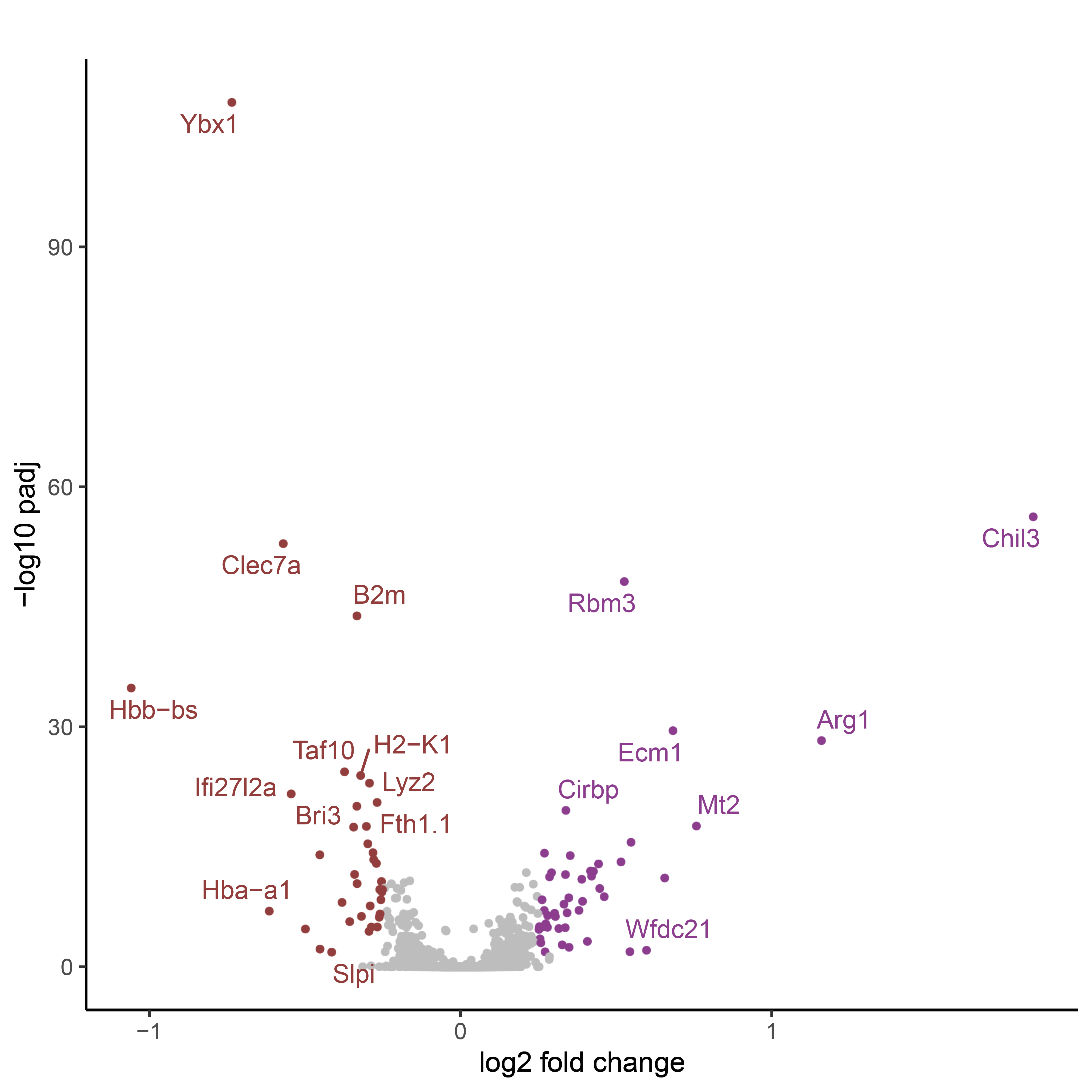
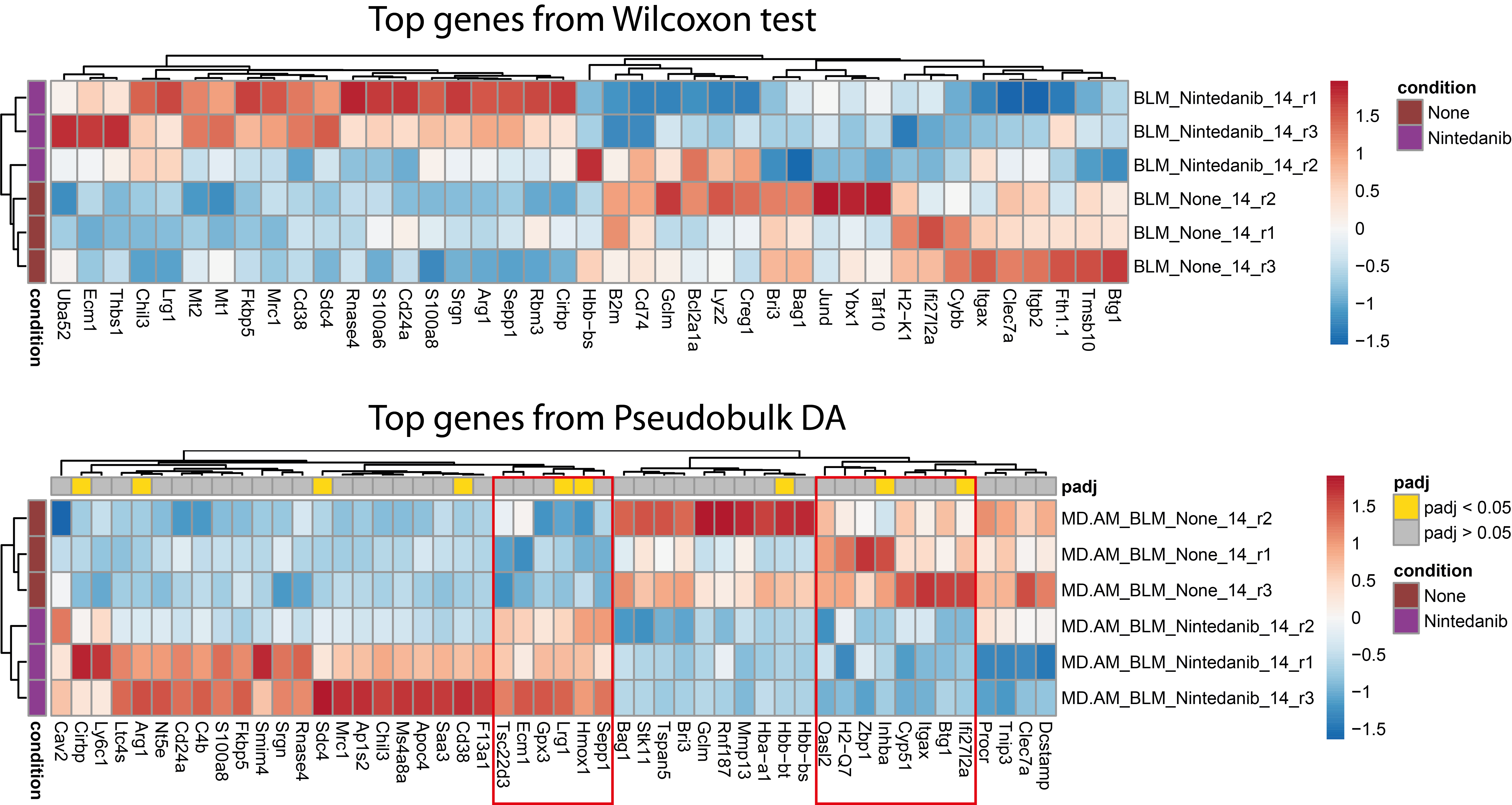
In order to look for inconsistencies between biological replicates, plot the heatmap of the per-sample mean gene expression for the top most differentially expressed genes.

# Select the top 50 genes with the smallest adjusted pvalue
df <- gene_list %>% top_n(50,-log10(p_val_adj))

# Compute their mean expression of Nintedanib-treated or untreated TR-AM in each sample
data <- aggr %>% subset(subset=celltype == "TR-AM" & group %in% c("BLM_Nintedanib_d14","BLM_None_d14")  ) %>% AverageExpression(assays = "RNA",slot = "data",group.by ="sample",features = df$gene)

# Extract the corresponding count matrix
data <- data[["RNA"]]

# Create an annotation dataframe which specifies the corresponding condition of each sample
# The rownames of it must be in the same order than the colnames of the data matrix
annotation <- data.frame(row.names = colnames(data),condition = ifelse(grepl('None', colnames(data)), 'None', 'Nintedanib'))

# Use this function to scale the data = compute z-scores (it retrieves the cell-wise mean to each value and divides by the cell-wise standard deviation)
data <- flexible_normalization(data)

# List the color of the annotation to display in the heatmap
annot.cols <- list("condition"=c("None"="#913c3c","Nintedanib"="#8e3c91"))

# Create a color palette for the scaled gene expression, with the white centered on 0 values
paletteLength = 100
myColor = colorRampPalette(rev(brewer.pal(n = 9, name ="RdBu")))(paletteLength)
Breaks = c(seq(min(data), 0, length.out=ceiling(paletteLength/2) + 1),
           seq(max(data)/paletteLength, max(data), length.out=floor(paletteLength/2)))

p1 <- pheatmap(t(data),annotation_row = annotation,annotation_colors = annot.cols,cluster_cols = T,cluster_rows = T,color = myColor,fontsize_col =10,treeheight_row = 10,treeheight_col = 10,breaks = Breaks,show_colnames = T)

2. Method n°2 : Wilcoxon test on single-cell profiles

When comparing conditions that include cells from multiple independent samples, it is recommended to use tools designed for DEA on bulk RNA-seq data. Their statistical models are more reliable because they account for biological variability between replicates and allow for the addition of cofactors. To mimic bulk RNA-seq data which add up counts of multiple cells, the idea is to create "pseudo-bulks" by aggregating raw counts from a homogeneous population of cells from the same sample. The pseudo-bulks corresponding to the same cell population and experimental condition are inputs of DEA tools such as DESeq2 or edgeR, where they're considered as biological replicates.

2.1 Construct pseudobulks

Although comparative studies have shown that this approach outperforms methods dedicated to scRNA-seq data analysis, its performance depends on several factors, including the number of pseudobulks replicates in each compared condition, the number of aggregated counts per pseudobulk, and of course the magnitude and stability of the gene expression modulation being quantified.

Furthermore, it is essential that the number of cells used to construct pseudo-bulks is sufficient (100 cells minimum), and that it is equivalent between each sample, to avoid detecting differences in expression due to an imbalance in the number of aggregated counts.

# Load DESeq2 package and the seurat object
library(DESeq2)
aggr <- readRDS("/data/analysis/data_truchi/GSE151374_Final.rds")

# Define the metadata variable that identify each sample 
aggr$identifier <- aggr$sample

# Construct the pseudobulk matrix that aggregates the raw counts of cells from the same celltype and identifier
cts <- AggregateExpression(aggr,group.by = c("celltype","identifier"),return.seurat = F,assays = "RNA",slot = "counts")

# Transform the matrix to fit with DESeq2 data structure
cts <- t(cts$RNA) %>% as.data.frame()

# Split the matrix by celltype
splitRows <- gsub('_.*', '', rownames(cts))
cts.split <- split.data.frame(cts, f = factor(splitRows))
cts.split <- lapply(cts.split, function(x){ 
  t(x)})

2.2 Perform DEA with DESeq2

Once pseudobulks counts matrix are made for each celltype, they can be use as inputs of DESeq2 DEA workflow. Briefly, counts are first normalized for each pseudobulk using the median of ratios obtained by dividing the counts of each gene in the pseudobulk by the average counts of the same gene across the entire dataset. The dispersion of each gene is then estimated using maximum likelihood and related to the mean of its normalized counts. The observed dispersion of each gene is corrected based on its deviation from the expected dispersion according to the model. This correction is increased when the number of samples is low, and genes with observed dispersion far exceeding the expected dispersion are not corrected to avoid introducing noise into the model. This approach accounts for variability between samples, preventing technical variations from being detected as biological variations. Each count is modeled using a negative binomial probability law parameterized with its normalization coefficient and corrected dispersion. A Wald test is performed to determine if the hypothesis of equal expression between the two compared groups can be rejected. The associated p-values are corrected for multiple testing using the Benjamini-Hochberg method. The magnitude of the variation is calculated using a log2 fold change, which is the log2 of the ratio between the mean modeled counts in the first group and the second group.

We run this workflow to compare TR-AM of Nintedanib-treated mice to TR-AM of untreated mice.

# Extract the counts of TR-AM from "BLM_None_14"and "BLM_Nintedanib_14" samples
cts <- cts.split$`TR-AM`
cts <- cts[,grepl(pattern = 'BLM_None_14|BLM_Nintedanib_14', x = colnames(cts))]

# Create an annotation dataframe specifying the condition of each sample
colData <- data.frame(identifier = colnames(cts)) %>% mutate(condition = ifelse(grepl('Nintedanib', identifier), 'Nintedanib', 'None')) 
colData$condition <- factor(colData$condition,levels = c('None', 'Nintedanib'))

# Create a DESeqDataSetFromMatrix object linking the count matrix and the annotation
# Specify the design of the DEA, that is comparing the entities from the "condition" annotation column
dds <- DESeqDataSetFromMatrix(countData = cts,colData = colData,design = ~ condition)

# Remove genes with less than 10 aggregated counts in all compared pseudobulks
dds <- dds[rowSums(counts(dds)) >=10,]

# Run the DEA
dds <- DESeq(dds)

# Look at the different contrasts
resultsNames(dds)

# Extract a specific contrast
DEA_m2 <- results(dds, contrast=c("condition", "Nintedanib", "None"), parallel=TRUE)%>% as.data.frame()%>% mutate(gene=rownames(.))%>% mutate(test="Nintedanib_vs_None")

# Write the DEA table
write.xlsx(DEA_m2,file="DEA_table_DESeq2.xlsx")

2.3 Represent differentially expressed genes

Select only genes considered as signifcantly up or downregulated based on LFC and adjusted pvalues thresholds. Display them in a volcano plot.

gene_list_2 <- DEA_m2 %>% filter(baseMean > 25)
upgene_Bleo <- gene_list_2 %>% arrange(dplyr::desc(log2FoldChange)) %>% filter(log2FoldChange > 0.25 & padj<0.05)  %>% na.omit() %>% pull(gene)
dwgene_Bleo <- arrange(gene_list_2, log2FoldChange) %>% filter(log2FoldChange < -0.25 & padj<0.05)  %>%  na.omit() %>% pull(gene)
genestoshow_2 <- c(upgene_Bleo, dwgene_Bleo)
print(genestoshow_2)

gene_list_2$gene <- ifelse(gene_list_2$gene %in% genestoshow_2, gene_list_2$gene, "")

# Define a label for down-regulated, up-regulated, and not significant genes
gene_list_2$threshold = as.factor(ifelse(gene_list_2$padj > 0.05, 'not significant', 
                                         ifelse(gene_list_2$padj < 0.05 & gene_list_2$log2FoldChange <= -0.25, 'down-regulated',
                                                ifelse(gene_list_2$padj < 0.05 & gene_list_2$log2FoldChange >= 0.25, 'up-regulated', 'not significant'))))

ggplot(gene_list_2, aes(x=log2FoldChange, y=-log10(padj))) +
  ggrastr::geom_point_rast(aes(color = threshold), shape = 20, alpha = 1, size = 1.25) +
  scale_x_continuous(limits = c(-3.5, 3)) +
  scale_color_manual(values = c("#913c3c", 'grey', "#8e3c91")) +
  ggtitle("") +
  xlab("log2 fold change") + ylab("-log10 padj") +
  #geom_hline(yintercept = -log10(0.05), colour="#990000", linetype="dashed") + geom_vline(xintercept = 0.5, colour="#990000", linetype="dashed") + geom_vline(xintercept = -0.5, colour="#990000", linetype="dashed") +
  theme_classic() + 
  theme(legend.position = "none") +
  geom_text_repel(data=filter(gene_list_2, padj<0.05), aes(label = gene, color = threshold), size = 3.5)

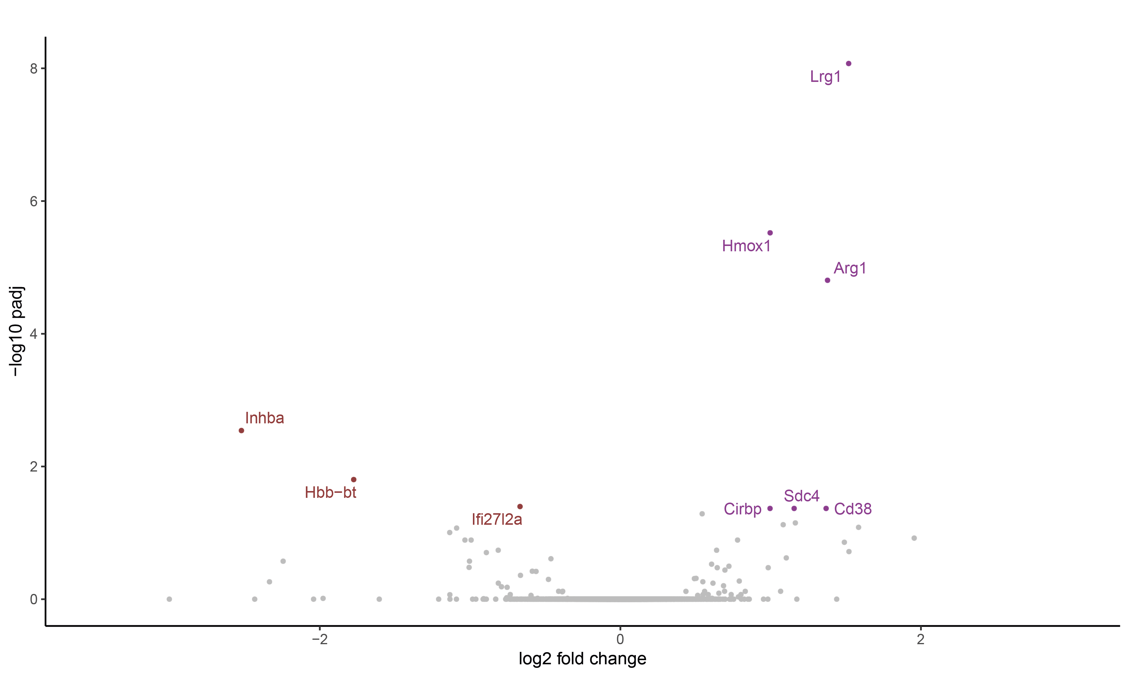
As we can see, the pseudobulk approach is much more stringent, as it has found only 10 differentially expressed genes with an adjusted pvalue under the 0.05 threshold.
These poor results can be explained by the small number of samples compared (3 Nintedanib vs 3 untreated), or by the heterogeneity of the modulation.

To take a closer look at the DEA results, plot the heatmap of the per-sample mean gene expression for the top most differentially expressed genes based on non-adjusted pvalue.

# Select the top 50 genes with the smallest adjusted pvalue
df <- gene_list_2 %>% top_n(50,-log10(pvalue))

# Extract the corresponding pseudobulk count matrix
data <- data.frame(counts(dds, normalized=TRUE))[rownames(df),]  %>% as.data.frame() 

# Create an annotation dataframe which specifies the corresponding condition of each sample
# The rownames of it must be in the same order than the colnames of the data matrix
annotation <- dds@colData %>% as.data.frame()%>% dplyr::select(condition)
rownames(annotation) <- gsub("-",".",rownames(annotation))

# Create also an annotation for the gene, in order to highlight those with a significant adjusted pvalue 
gene.annotation <- data.frame(row.names = rownames(data),padj= ifelse(rownames(data) %in% c(gene_list_2 %>% filter(padj<0.05) %>% pull(gene)),"padj < 0.05","padj > 0.05"))

# Use this function to scale the data = compute z-scores (it retrieves the cell-wise mean to each value and divides by the cell-wise standard deviation)
data <- flexible_normalization(data)

# List the color of the columns and rows annotation to display in the heatmap
annot.cols <- list("condition"=c("None"="#913c3c","Nintedanib"="#8e3c91"), "padj" =c("padj < 0.05"="gold","padj > 0.05"="grey"))

# Create a color palette for the scaled gene expression, with the white centered on 0 values
paletteLength = 100
myColor = colorRampPalette(rev(brewer.pal(n = 9, name ="RdBu")))(paletteLength)
Breaks = c(seq(min(data), 0, length.out=ceiling(paletteLength/2) + 1),
           seq(max(data)/paletteLength, max(data), length.out=floor(paletteLength/2)))

p2 <- pheatmap(t(data),annotation_row = annotation,annotation_col = gene.annotation,annotation_colors = annot.cols,cluster_cols = T,cluster_rows = T,color = myColor,fontsize_col = 10,treeheight_row = 10,treeheight_col = 10,breaks = Breaks,show_colnames = T)

By comparing both heatmaps visually, it appears that the signature identified with pseudobulks is more consistent across biological replicates than that obtained via the Wilcoxon test (see the genes highlighted in the red boxes). This comparison illustrates the limitations of examinating results solely on the basis of pvalues and their adjustment.

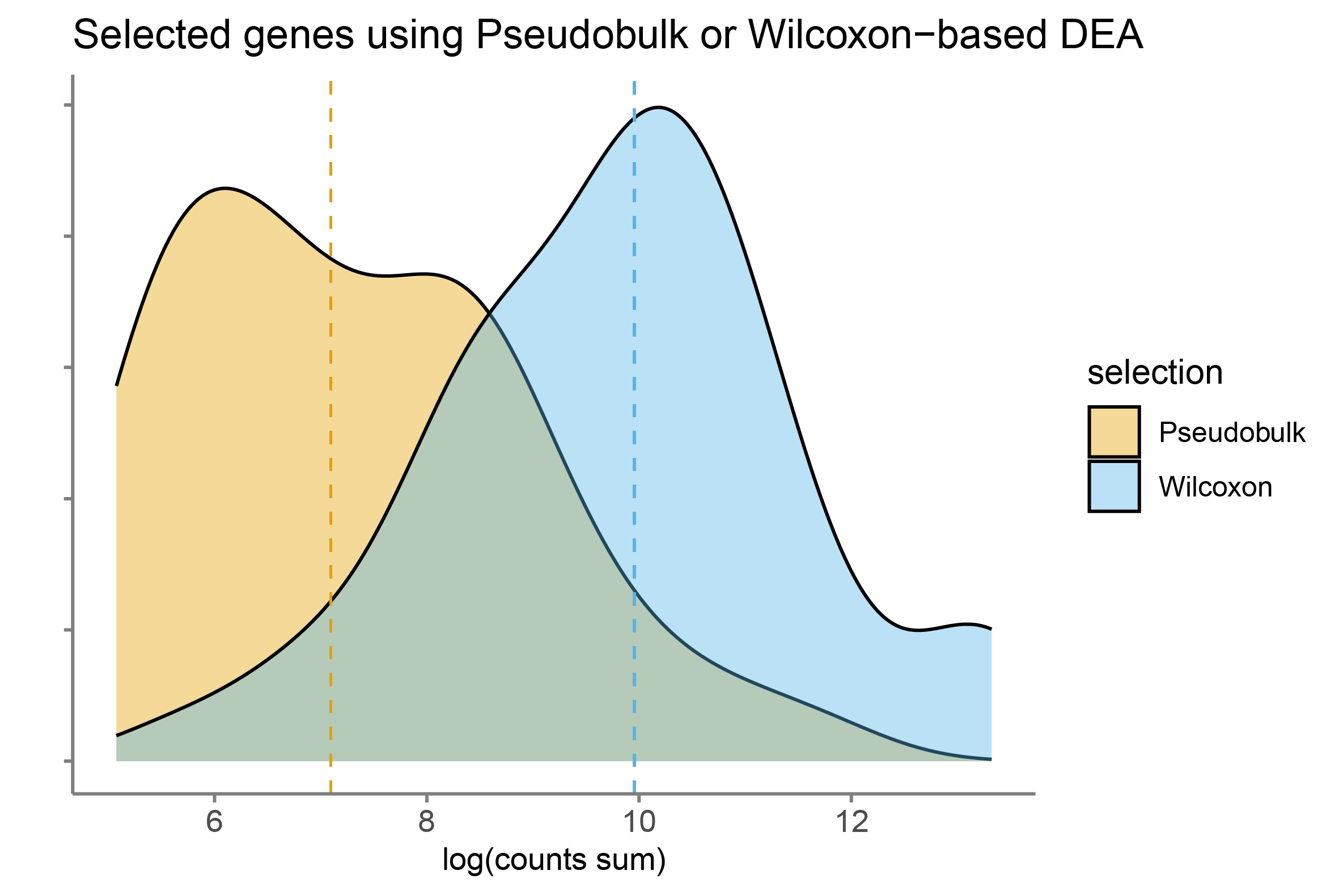
Also, when we compare the top 50 differentially expressed genes with the smallest pvalue identified using the Pseudobulk-based or the Wilcoxon-based approach, we observed than the Pseufobulk approach tends to select lower expressed genes.
On one hand, it can be seen as a positive feature that prevent detecting genes with a high mean-to-variance relation.
However, it may also favors the detection of lowly-expressed genes that are noisy, such as ambient RNA or other ectopic molecules.

Differential Expression Analysis

Module specifications

Code