MS_based_lipidomics-Peak_area_analysis
Lipidomics Bulk Statistical analysisThis module shows how to use Lipidr, a R/Bioconductor package designed for the analysis of quantitative MS-based lipidomics datasets. First, sample information and lipid quantification matrix are processed to build a LipidExperiment object that integrates lipid annotations. After quality control checks, the data are normalized using PQN to ensure balanced peak area across samples. Sample correlations and PCA are used to explore relationships between samples. Finaly OPLS-DA and differential analysis based on limma are performed to identify differentially expressed lipids between conditions, which are represented in heatmaps and volcano plots.
Module specifications
| Input data | Computational environnement | Output data |
|---|---|---|
|
LipidSearch output |
Lipidomics_data_analysis R |
differential analysis table |
Code
None
This module is based on the following documentation :
LipidR bioconductor package
Mohamed A, Molendijk J, Hill MM. lipidr: A Software Tool for Data Mining and Analysis of Lipidomics Datasets. J Proteome Res. 2020;19(7):2890-2897. doi:10.1021/acs.jproteome.0c00082
* https://pubmed.ncbi.nlm.nih.gov/32168452/
* https://www.bioconductor.org/packages/release/bioc/vignettes/lipidr/inst/doc/workflow.html
This module require to load the following environment of R packages :
source("lipidomics_R_packages.R")
Informations about the demo dataset :
The demo dataset is the result of the quantification of 112 lipids in 160 samples, splitted in two groups, obtained with the LipidSearch (v5.0) software (https://assets.thermofisher.com/TFS-Assets/CMD/posters/PO-65031-LC-MS-Lipidomics-LipidSearch-ASMS2017-PO65031-EN.pdf).
LipidSearch pre-processing involves detecting peaks by analyzing raw mass spectrometry files to determine accurate masses of MSn and precursor ions. It identifies lipids by searching a large database of predicted lipid structures and ion adducts to match candidate molecular species. The process aligns search results from individual samples within a time window into a single report and quantifies accurate-mass extracted ion chromatograms to obtain peak areas for each identified lipid precursor.
Notes
lipidr implements a series of functions to perform quality control, differential analysis, multivariate statistics, lipid set enrichment and chain trend analysis
It is not the only R package dedicated to lipidomics data analysis, but it seems the most used workflow, notably cited in https://pubmed.ncbi.nlm.nih.gov/37904045/ & https://pubmed.ncbi.nlm.nih.gov/37075753/, and is well maintained.
1. Prepare data to build a LipidExperiment object
1.1 Prepare the sample annotation table
A simple annotation table, with ordered condition levels for visualization purposes.
## read samples information from external file
metadata_file <- read.xlsx("namefile.xlsx")
metadata_file$Sample_name <- gsub("([^.]+)[_].*", "\\1", metadata_file$File.Name)
metadata_file$Condition <- gsub("-.*","",metadata_file$Sample_name)
metadata_file$Condition <- ifelse(startsWith(metadata_file$Condition, "M"), "M", metadata_file$Condition)
metadata_file$Condition <- ifelse(startsWith(metadata_file$Condition, "O"), "O", metadata_file$Condition)

## order it for plotting
metadata_file$Condition <- factor(metadata_file$Condition,levels = c(unique(metadata_file$Condition)))

metadata_file <- metadata_file %>% arrange(Condition) %>% as.data.table()
## define the technical replicates
metadata_file[ , tech_repl := 1:.N , by = c("Sample_name") ]
1.2 Read the peak area table and process it
Read the peak area table produced by LipidSearch, displayed here as a .txt file.
LSoutput = read.table("merged_table.txt",sep = "\t",header = T)
Save LipidSearch nomenclature of lipids for further processing.
LSN <- LSoutput %>% mutate(Peptide=LipidID) %>% dplyr::select(Peptide,LipidID,Class, SubClass, IonFormula)
Transform the LipidSearch output in a dataframe of area values where the first column in named "Peptide" (this is strange but it is needed to further handle the dataset in a specific format).
LSoutput <- LSoutput %>% mutate(Peptide=LipidID) %>% dplyr::select(Peptide,metadata_file$Arbitrary_name )
Take the median of values across technical replicate.
LSoutput_t <- LSoutput %>% mutate(Peptide=make.unique(Peptide)) %>% column_to_rownames(.,"Peptide") %>% t() %>% as.data.frame()
LSoutput_t <- merge(metadata_file %>% dplyr::select(Arbitrary_name,renamed_sample_name) %>% column_to_rownames(.,"Arbitrary_name"),LSoutput_t,by="row.names") %>% column_to_rownames(.,"Row.names")
LSoutput_t <- LSoutput_t %>% dplyr::group_by(renamed_sample_name) %>% dplyr::summarise(across(everything(), \(x) median(x, na.rm = TRUE)))
LSoutput <- LSoutput_t %>% column_to_rownames(.,"renamed_sample_name") %>% t() %>% as.data.frame() %>% mutate(Peptide=rownames(.)) %>% relocate(Peptide, .before =1)
Remove technical replicates from metadata.
metadata_file <- metadata_file %>% mutate(Sample=renamed_sample_name) %>% dplyr::select(Sample,Condition) %>% unique() %>% as.data.frame()
metadata_file <- metadata_file[match(colnames(LSoutput[,-1]),metadata_file$Sample),]
metadata_file$Sample <- factor(metadata_file$Sample,levels = c(metadata_file$Sample))
rownames(metadata_file) <- metadata_file$Sample
Remove Lipids which have no quantification in at least 25% of samples from a particular condition.
LSoutput_t <- LSoutput %>% dplyr::select(-Peptide) %>% t() %>% as.data.frame()
LSoutput_t <- merge(metadata_file %>% dplyr::select(Condition),LSoutput_t,by="row.names") %>% column_to_rownames(.,"Row.names")
LSoutput_t <- LSoutput_t %>% dplyr::group_by(Condition) %>% dplyr::summarise(across(everything(), ~ sum(is.na(.))))
LSoutput_t <- cbind(Condition=LSoutput_t$Condition,sweep(LSoutput_t %>% dplyr::select(-Condition), 1, table(metadata_file$Condition), `/`) )
LSoutput_t <- LSoutput_t %>% pivot_longer(-Condition,names_to="Lipids",values_to="values")
lipids_to_remove <- LSoutput_t %>% filter(values > 0.25) %>% pull(Lipids)

LSoutput <- LSoutput %>% filter(Peptide %ni% lipids_to_remove)
LSN <- LSN %>% filter(Peptide %ni% lipids_to_remove)
Remove suffixes to Peptides names and rownames.
LSN$Peptide <- gsub("\\..*","",LSN$Peptide)
LSoutput$Peptide <- gsub("\\..*","",LSoutput$Peptide)
rownames(LSoutput) <- NULL
Check if samples are in the same order in the Area matrix and the metadata.
all(colnames(LSoutput %>% dplyr::select(-Peptide))==metadata_file$Sample)
LSoutput <- LSoutput[,match(c("Peptide",as.character(metadata_file$Sample)),colnames(LSoutput))]
all(colnames(LSoutput %>% dplyr::select(-Peptide))==metadata_file$Sample)
Remove the additional group after peptide name, it is not recognized by lipidR, whereas it is important to keep as it defines the lipid identity.
LSoutput$Peptide <- gsub("\\+.*","",LSoutput$Peptide)
# but keep it in the LSN table
# LSN$Peptide <- gsub("\\+.*","",LSN$Peptide)
Convert to Lipidomics Experiment Object, an annotated matrix format that combine sample information and quantitative information.
During the convertion, lipidR will parse the lipid nomenclature if it recognizes the pattern ( it automatically adds lipid class, number of chain, number of carbones, number of saturations ...).
LipidExp<- as_lipidomics_experiment(LSoutput, logged = FALSE, normalized = FALSE)
2. Finalize the LipidExperiment object
2.1 Fill missing information on lipid annotation
Add a class for lipids that has not been recognized by the lipidR parser.
rowData(LipidExp)$Class <- ifelse(is.na(rowData(LipidExp)$Class),gsub("\\(.*","",rowData(LipidExp)$Molecule),rowData(LipidExp)$Class)
Check which molecules have not been parsed (they will still be included in the differential analysis and plots).
annot <- lipidr::annotate_lipids(LSoutput[[1]])
Manually add the number of carbon and the number of double bonds per chain.
nchain <- strsplit(gsub("[^0-9:_]", "\\1", gsub(".*[(]([^.]+)[)].*", "\\1", rowData(LipidExp)$Molecule)), "_")
for (i in 1:length(nchain)) {
  rowData(LipidExp)$chain1[i] <- nchain[[i]][1]
  rowData(LipidExp)$chain2[i] <- nchain[[i]][2]
  rowData(LipidExp)$chain3[i] <- nchain[[i]][3]
  rowData(LipidExp)$chain4[i] <- nchain[[i]][4]
}
rowData(LipidExp)$l_1 <- ifelse(is.na(rowData(LipidExp)$l_1),gsub(":.*","",rowData(LipidExp)$chain1),rowData(LipidExp)$l_1) %>% as.numeric()
rowData(LipidExp)$s_1 <- ifelse(is.na(rowData(LipidExp)$s_1),gsub(".*:","",rowData(LipidExp)$chain1),rowData(LipidExp)$s_1) %>% as.numeric()
rowData(LipidExp)$l_2 <- ifelse(is.na(rowData(LipidExp)$l_2),gsub(":.*","",rowData(LipidExp)$chain2),rowData(LipidExp)$l_2) %>% as.numeric()
rowData(LipidExp)$s_2 <- ifelse(is.na(rowData(LipidExp)$s_2),gsub(".*:","",rowData(LipidExp)$chain2),rowData(LipidExp)$s_2) %>% as.numeric()
rowData(LipidExp)$l_3 <- ifelse(is.na(rowData(LipidExp)$l_3),gsub(":.*","",rowData(LipidExp)$chain3),rowData(LipidExp)$l_3) %>% as.numeric()
rowData(LipidExp)$s_3 <- ifelse(is.na(rowData(LipidExp)$s_3),gsub(".*:","",rowData(LipidExp)$chain3),rowData(LipidExp)$s_3) %>% as.numeric()

rowData(LipidExp)$total_cl <- ifelse(is.na(rowData(LipidExp)$total_cl),mapply(sum, rowData(LipidExp)$l_1, rowData(LipidExp)$l_2, rowData(LipidExp)$l_3,rowData(LipidExp)$l_4, na.rm=TRUE),rowData(LipidExp)$total_cl)
rowData(LipidExp)$total_cs <- ifelse(is.na(rowData(LipidExp)$total_cs),mapply(sum, rowData(LipidExp)$s_1, rowData(LipidExp)$s_2, rowData(LipidExp)$s_3,rowData(LipidExp)$s_4, na.rm=TRUE),rowData(LipidExp)$total_cs)
Replace lipidR nomenclature by LipidSearch nomenclature.
LipidExp@elementMetadata@listData[["clean_name"]] <- LSN$LipidID
2.2 Add sample annotation to the LipidExperiment object
It requires writing the sample annotation as .csv file, which is then loaded.
All samples names must be in the first column or in a column named "Sample".
write.csv(metadata_file %>% mutate(Sample_name=Sample),"./metadata.csv",row.names = F)
LipidExp = add_sample_annotation(LipidExp, "./metadata.csv")
colData(LipidExp)
Finally, order conditions and samples for plotting.
LipidExp$Condition <- factor(LipidExp$Condition,levels = c(unique(metadata_file$Condition) ))
LipidExp$Sample_name <- factor(LipidExp$Sample_name,levels = c(metadata_file$Sample))
3. Quality control and Normalization
3.1 Check the quantification differences between samples and lipids groups
The raw number of peak area should be unbalanced between samples.
# set a color palette for conditions
col.cond <- c("M"="#71a659","O"="#8975ca")
# plot the total peak area per sample as bar chart or the per-lipid distribution within each samples as a boxplot
plot_samples(LipidExp, type = "tic", log = TRUE,color = "Condition")+scale_fill_manual(values = col.cond)
plot_samples(LipidExp, type = "boxplot", log = TRUE,color = "Condition")+scale_fill_manual(values = col.cond)
Create a dataframe for plotting peak area for each lipid grouped per condition/ per class.
df <- LipidExp@assays@data@listData[["Area"]]
df <- df %>% as.data.frame() %>% mutate(clean_name=LipidExp@elementMetadata@listData[["clean_name"]])
df <- cbind(df,LSN %>% dplyr::select(-Peptide))
df <- df %>% pivot_longer(-c("clean_name","LipidID","Class","SubClass","IonFormula"),names_to="Sample",values_to="Area")

df <- inner_join(df,metadata_file)
df$Area_log2 <- log2(df$Area+1)

ggboxplot(df %>% filter(Class=="Cer"), x="clean_name",y= "Area_log2",fill = "Class",ylab = "Area",outlier.shape = NA) + theme(axis.text.x = element_text(size = 10, angle = 90))
3.2 Optionnaly input NA values and summarize transitions
Some NA values, corresponding to technical bias, can be imputted according to several methods, such as "knn" which input the average values found in the k nearest neighbors of the particular sample.
LipidExp <- impute_na(LipidExp,measure = "Area",method = "knn",10)
This step is important when more than one transition is measured per lipid molecule. Multiple transitions are summarized into a single value by either taking the average intensity or the one with highest intensity.
If there is no duplication, running the function will return an error.
## Which Lipid name is duplicated ?
LipidExp@elementMetadata@listData[["clean_name"]][duplicated(LipidExp@elementMetadata@listData[["clean_name"]])==TRUE]

LipidExp = summarize_transitions(LipidExp)
3.3 Normalize data to obtain a balanced peak area average for all samples
The Probabilistic Quotient Normalization (PQN) method determines a dilution factor for each sample, by comparing the distribution of quotients between samples and a reference spectrum, followed by sample normalization using this dilution factor.
The reference spectrum in this method is the average lipid abundance of all samples.
LipidExp_norm = normalize_pqn(LipidExp, measure = "Area", exclude = "blank", log = TRUE)
plot_samples(LipidExp_norm, type = "tic", log = TRUE,color = "Condition")+scale_fill_manual(values = col.cond)
plot_samples(LipidExp_norm, type = "boxplot", log = TRUE,color = "Condition")+scale_fill_manual(values = col.cond)

# add lipid name as rownames of the Area matrix, which are numbers by default
rownames(LipidExp_norm@assays@data@listData[["Area"]]) <- LipidExp_norm@elementMetadata@listData[["clean_name"]]
3.4 Explore the global relationships between samples (Correlation and PCA)
Plot a Heatmap or Pearson's correlation coefficients between samples.
data <- LipidExp_norm@assays@data@listData[["Area"]]
cm <- cor( na.omit(data))
# rearrange columns so that same sample types are together
annotation <- data.frame(row.names=colnames(cm),condition=ifelse(startsWith(colnames(cm), "O"), "O", "M"))
pheatmap(cm,cluster_rows=T, cluster_cols=T,annotation_col = annotation,annotation_colors = list("condition"=col.cond),
         color = hcl.colors(20, palette = "Viridis"))
Run PCA to investigate overall variability of the dataset.
mvaresults = mva(LipidExp_norm, measure="Area", method="PCA")
pca_df <- mvaresults[["scores"]] %>% dplyr::select(p1,p2) %>% mutate(Sample=rownames(.)) %>% inner_join(metadata_file)

ggplot(pca_df, aes(x = p1, y = p2, fill = Condition)) +
  geom_point(shape=21,alpha=2,  size=2)+
  ggtitle("PCA")+stat_ellipse(geom="polygon", aes(fill = Condition), alpha = 0.2,show.legend = FALSE, level = 0.95)+
  scale_fill_manual(values = col.cond) +
  theme_minimal() + xlab(paste0("PC1: ",mvaresults[["summary"]]["p1","R2X"]*100,"%")) + ylab(paste0("PC2: ",mvaresults[["summary"]]["p2","R2X"]*100,"%"))+
  theme(axis.text.x = element_text(size = 10, angle = 0),
        axis.title.y = element_text(size = 10),
        axis.title.x = element_text(size = 10),
        axis.text.y = element_text(size = 10, angle = 90),
        axis.line = element_line(colour = "grey50"),
        axis.ticks = element_line(colour = "grey50"),
        legend.text = element_text(size = 12),
        legend.title = element_text(size = 12))
4. Identify differentially detected lipids between conditions
4.1 Supervised multivariate analysis (OPLS-DA)
Orthogonal Partial Least Squares-Discriminant Analysis (OPLS-DA) is a multivariate statistical method used to select features discriminating groups of samples. It extends Partial Least Squares (PLS) regression by separating the variation in the data into predictive and orthogonal (non-predictive) components, enhancing the interpretation of the model by focusing on the differences between groups.
mvaresults = mva(LipidExp_norm, method = "OPLS-DA", group_col = "Condition", groups=c("M", "O"))
opls_da_MvsO <- top_lipids(mvaresults, top.n=length(mvaresults[["row_data"]]@rownames))
Plot the heatmap of peak area of top PLS-DA selected lipids.
data <- LipidExp_norm@assays@data@listData[["Area"]]
data <- data %>% as.data.frame()
rownames(data) <- LipidExp_norm@elementMetadata@listData[["clean_name"]]
data <- data[opls_da_MvsO$clean_name, metadata_file %>% dplyr::filter(Condition %in% c("M", "O"))%>% pull(Sample)]
data <- flexible_normalization(data)
data[data>3] <- 3
data[data < -3] <- -3
annotation <- data.frame(row.names=colnames(data),Sample=colnames(data))
annotation <- inner_join(annotation,metadata_file %>% dplyr::select(Sample,Condition)) %>% column_to_rownames(.,"Sample")
pheatmap(data,show_colnames = T,show_rownames = T,cluster_cols = T,cluster_rows = T,treeheight_row = 0,treeheight_col = 0,legend = T,annotation = annotation,annotation_colors = list(Condition=col.cond),
         color = colorRampPalette(rev(brewer.pal(n = 9, name ="RdBu")))(100),annotation_legend = T,angle_col = 90,number_color="black",number_format="%.f")
4.2 Perform classical differential analysis
The statistical framework used by lipidR is based on limma, a widely-used R package for microarray data analysis (Smyth G. et al 2004).
Nomenclature <- LipidExp_norm@elementMetadata@listData[["clean_name"]]
LipidExp_norm@elementMetadata@listData[["Molecule"]] <- factor(Nomenclature,levels=Nomenclature)
de_results_MvsO <-  de_analysis(data=LipidExp_norm,group_col="Condition", M - O,measure="Area") %>% mutate(log10padj=-log10(adj.P.Val))
de_results_MvsO <- inner_join(LSN %>% mutate(Molecule=LipidID) %>% dplyr::select(Molecule,SubClass,IonFormula) %>% unique(),de_results_MvsO) %>% arrange(adj.P.Val)
de_results_MvsO <- de_results_MvsO %>% inner_join(opls_da_MvsO %>% mutate(opls_rank=molrank, Molecule=clean_name )%>% dplyr::select(Molecule ,opls_rank))

# Write the differential analysis table
write.xlsx(de_results_MvsO,file = "./lipidR_DA_vetagro.xlsx")
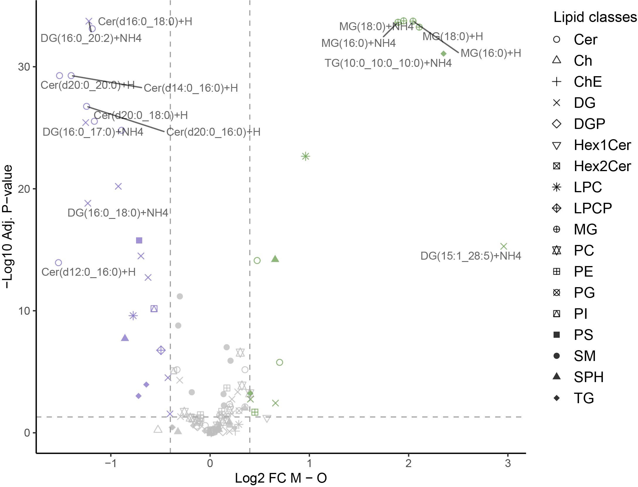
4.2 Plot the results of the differential analysis
Volcano plots where lipids showing an absolute log2FC and an ajusted pvalue passing the defined thresholds are highlighted.
If there are no lipids satisfying the condition, the graph may not be displayed correctly.
# Classic
lipidr_volcano(de_results = de_results_MvsO,maxAdjP = 0.05,minFC = 0.4,contrast_to_plot = "M - O",lipids_to_show = 20,cols = c("#71a659","#8975ca"))
# On particular lipid classes
selected_class <- c("MG","DG","Cer")
lipidr_volcano(de_results = de_results_MvsO,selected_class = selected_class,maxAdjP = 0.05,minFC = 0.4,contrast_to_plot = "M - O",lipids_to_show = 20,cols = c("#71a659","#8975ca"))
# Colored by the total number of carbons
lipidr_volcano(de_results = de_results_MvsO,by.cl = T,maxAdjP = 0.05,minFC = 0.4,contrast_to_plot = "M - O",lipids_to_show = 20,cols = c("#71a659","#8975ca"))
lipidr_volcano(de_results = de_results_MvsO,by.cl = T,selected_class = selected_class,maxAdjP = 0.05,minFC = 0.4,contrast_to_plot = "M - O",lipids_to_show = 10,cols = c("#71a659","#8975ca"))
Heatmap of top differentially expressed lipids.
data <- LipidExp_norm@assays@data@listData[["Area"]]
data <- data %>% as.data.frame()
rownames(data) <- LipidExp_norm@elementMetadata@listData[["clean_name"]]

selected.lipids <- de_results_MvsO %>% filter(contrast %in% c("M - O") & adj.P.Val<= 0.05 & abs(de_results_MvsO$logFC)>0.4)
data <- data[selected.lipids$Molecule, metadata_file %>% dplyr::filter(Condition %in% c("M", "O"))%>% pull(Sample)]
data <- flexible_normalization(data)
data[data>3] <- 3
data[data < -3] <- -3

annotation_col <- data.frame(row.names=colnames(data),Sample=colnames(data))
annotation_col <- inner_join(annotation_col,metadata_file %>% dplyr::select(Sample,Condition)) %>% column_to_rownames(.,"Sample")
annotation_row <- data.frame(row.names=rownames(data),Class=selected.lipids$Class)
class.col <- color_scheme$hex(unique(de_results_MvsO$Class) %>% length())
names(class.col) <- unique(de_results_MvsO$Class)
pheatmap(data,show_colnames = T,show_rownames = T,cluster_cols = T,cluster_rows = T,treeheight_row = 0,treeheight_col = 0,legend = F,
         annotation = annotation_col,annotation_row = annotation_row,annotation_colors = list(Condition=col.cond,Class=class.col),
         color = colorRampPalette(rev(brewer.pal(n = 9, name ="RdBu")))(100),annotation_legend = T,angle_col = 90,number_color="black",number_format="%.f")